Download presentation
Presentation is loading. Please wait.

1
Minimum Power Configuration in Wireless Sensor Networks Guoliang Xing*, Chenyang Lu*, Ying Zhang**, Qingfeng Huang**, and Robert Pless* *Washington University in St. Louis **Palo Alto Research Center (PARC) Inc. MobiHoc '05 Chien-Ku Lai
 Inc. MobiHoc 05 Chien-Ku Lai.")
2
Outline Introduction An Illustrating Example Problem Definition Approximation Algorithms Experimentation Discussion Conclusion

3
Introduction - Wireless Sensor Network (WSN) WSNs must aggressively conserve energy to operate for extensive periods Wireless communication often dominates the energy dissipation in a WSN Topology control Power-aware routing Sleep management Turning off redundant nodes Only keeping a small number of active nodes
 WSNs must aggressively conserve energy to operate for extensive periods Wireless communication often dominates the energy dissipation in a WSN Topology control Power-aware routing Sleep management Turning off redundant nodes Only keeping a small number of active nodes")
4
Introduction - Minimum Power Configuration (MPC) When network workload is low The power consumption of a WSN is dominated by the idle state Scheduling nodes to sleep saves the most power It is more power-efficient for active nodes to use long communication ranges When network workload is high Short radio ranges may be preferable
 When network workload is low The power consumption of a WSN is dominated by the idle state Scheduling nodes to sleep saves the most power It is more power-efficient for active nodes to use long communication ranges When network workload is high Short radio ranges may be preferable")
5
Introduction - Minimum Power Configuration (MPC) MPC provides a unified approach integrating Topology control Power-aware routing Sleep management
 MPC provides a unified approach integrating Topology control Power-aware routing Sleep management")
6
An Illustrating Example Two network configurations 1. a communicates with c directly using transmission range |ac| while b remains sleeping 2. a communicates with b using transmission range |ab| and b relays the data from a to c using transmission range |bc| a b c

7
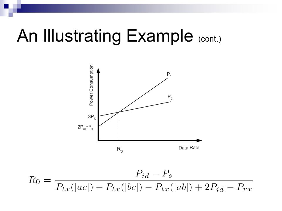
An Illustrating Example (cont.) a b c R : a needs to send data to c at the rate B : The bandwidth of all nodes
 a b c R : a needs to send data to c at the rate B : The bandwidth of all nodes")
8
An Illustrating Example (cont.) a b c
 a b c")
10
An Illustrating Example - Mica2 Energy Model 433MHz Mica2 radio : The bandwidth : 38.4Kbps 30 transmission power level Suppose : P tx (|ac|) = maximum transmission power (80.1mW) P tx (|ab|) = P tx (|bc|) = 24.6mW P id = 24mW P rx = 24mW P s = 6uW When R > 16.8Kbps Relaying through node b is more power efficient
 = maximum transmission power (80.1mW) P tx (|ab|) = P tx (|bc|) = 24.6mW P id = 24mW P rx = 24mW P s = 6uW When R > 16.8Kbps Relaying through node b is more power efficient")
11
Problem Definition A node can either be active or sleeping This work only considers the total active power consumption in a network The MPC problem : Given a network and a set of traffic demands, find a subnet that satisfies the traffic demands with minimum power consumption

12
Problem Definition (cont.) For the node u on the path f(s i,t j ) The data rate for source s i to sink t j
 For the node u on the path f(s i,t j ) The data rate for source s i to sink t j")
13
Problem Definition (cont.) Definition 1 (MPC problem)
 Definition 1 (MPC problem)")
14
Approximation Algorithms 1. Shortest-path Tree Heuristic (STH) 2. Incremental Shortest-path Tree Heuristic (ISTH)
.")
15
Shortest-path Tree Heuristic (STH)
")
16
2 22 2 2 2 2 2 1 3 4 2 4 2 1 s1s1 s2s2 t r1 = 0.1 r2 = 0.2

17
Shortest-path Tree Heuristic (STH) 2 22 2 2 2 2.2 2.1 2.3 2.4 2.2 2.4 2.2 2.1 s1s1 s2s2 t r1 = 0.1
 s1s1 s2s2 t r1 = 0.1")
18
Shortest-path Tree Heuristic (STH) 2 22 2 2 2 2.2 2.1 2.3 2.4 2.2 2.4 2.2 2.1 s1s1 s2s2 t r1 = 0.1
 s1s1 s2s2 t r1 = 0.1")
19
Shortest-path Tree Heuristic (STH) 2 22 2 2 2 2.4 2.2 2.6 2.8 2.4 2.82.4 2.2 s1s1 s2s2 t r2 = 0.2
 s1s1 s2s2 t r2 = 0.2")
20
Shortest-path Tree Heuristic (STH) 2 22 2 2 2 2.4 2.2 2.6 2.8 2.4 2.82.4 2.2 s1s1 s2s2 t r2 = 0.2
 s1s1 s2s2 t r2 = 0.2")
21
Incremental Shortest-path Tree Heuristic (ISTH)
")
22
2 22 2 2 2 2 2 1 3 4 2 4 2 1 s1s1 s2s2 t r1 = 0.1 r2 = 0.2

23
Incremental Shortest-path Tree Heuristic (ISTH) 2 22 2 2 2 2.2 2.1 2.3 2.4 2.2 2.4 2.2 2.1 s1s1 s2s2 t r1 = 0.1
 s1s1 s2s2 t r1 = 0.1")
24
Incremental Shortest-path Tree Heuristic (ISTH) 2 22 2 2 2 2.2 2.1 2.3 2.4 2.2 2.4 2.2 2.1 s1s1 s2s2 t r1 = 0.1
 s1s1 s2s2 t r1 = 0.1")
25
Incremental Shortest-path Tree Heuristic (ISTH) 2 22 2 2 2 2.4 0.4 2.2 2.6 2.8 2.4 2.8 0.4 2.2 s1s1 s2s2 t r2 = 0.2
 s1s1 s2s2 t r2 = 0.2")
26
Incremental Shortest-path Tree Heuristic (ISTH) 2 22 2 2 2 2.4 0.4 2.2 2.6 2.8 2.4 2.8 0.4 2.2 s1s1 s2s2 t r2 = 0.2
 s1s1 s2s2 t r2 = 0.2")
27
Experimentation 1. Simulation Environment 2. Simulation Settings 3. Results

28
Simulation Environment Simulator : Prowler The MAC layer in Prowler is similar to the B- MAC protocol in TinyOS

29
Simulation Settings MPCP is compared with two baseline protocols Minimum transmission ( MT ) routing Minimum transmission power ( MTP ) routing The number of nodes : 100 The region of network : 150m × 150m Divided into 10 × 10 grids Simulation time : 300s 60s for initialization phase
 routing Minimum transmission power ( MTP ) routing The number of nodes : 100 The region of network : 150m × 150m Divided into 10 × 10 grids Simulation time : 300s 60s for initialization phase")
30
Results - Total network energy cost

31
Results - Data delivery ratio at the sink

33
Discussion 1. Limitations of this paper 2. Potential future work

34
Discussion Every node in the network operates in a constant state Further energy savings can be achieved by reducing the idle time of active nodes

35
Discussion This approach mainly focuses on minimizing the total energy consumption Power-balanced should be achieved

36
Conclusion This paper proposes the minimum power configuration approach to minimize the total power consumption of WSNs formulates the energy conservation problem as a joint optimization problem where the power configuration of a network consists of a set of active nodes the transmission ranges of the nodes

37
Question? Thank you.

Similar presentations


 Octav Chipara Octav Chipara, Zhimin He, Guoliang Xing, Qin Chen, Xiaorui Wang, Chenyang.>")
 and prof. Christian Enz (EPFL-DE-LEG, CSEM) Wireless Sensor Networks:>")


 By Pakpoom Hoyingcharoen 3 November 2008 (2/2551)>")


