1. Lecture 5 More loops Introduction to maximum likelihood estimation Trevor A. Branch FISH 553 Advanced R School of Aquatic and Fishery Sciences University of Washington

2. More on loops Very often, we need to loop through a series of values, calculate something for each, and store the result General strategy – Find out how many iterations there will be ( niter ) – Make a vector of the values to loop over – Create a results vector of length niter – Loop from i in 1:niter – Conduct the analysis based on the i th element of values – Store the result in the i th element of results

3. Storing for-loop results, vector mean.norm <- function(n=c(5,10,15,30,50,100)) { niter <- length(n) values <- vector(length=niter) for (i in 1:niter) { values[i] <- sd(rnorm(n=n[i], mean=0, sd=1)) } return(values) } mean.norm() Number of iterations Create a vector to store the results Loop from 1 to niter, not over the set in n Store in the ith element of values Calculate using the ith element of n Return the vector of answers

4. Number of samples from rnorm(mean=0, sd=1) SD of samples

5. Storing for-loop results, matrix mean.norm.mat <- function(n=c(5,10,15,30,50,100), nrep=100) { niter <- length(n) values <- matrix(nrow=nrep, ncol=niter) for (i in 1:nrep) { for (j in 1:niter) { values[i,j] <- sd(rnorm(n=n[j], mean=0, sd=1)) } return(values) } x <- mean.norm.mat(nrep=1000) Create a matrix to store the results Return the matrix of answers Add another loop for nrep Side note: this is not necessarily the fastest way to program this

6. Histogram of standard deviations n = 5 n = 10 n = 15 n = 30 n = 50 n = 100

7. Fitting models to data Scenario: the length (L) of a fish is related to its age (a) according to the von Bertalanffy growth curve where is the asymptotic maximum length in cm, K is the growth rate, and t 0 is the age at zero length MalesFemales

8. One possible model fit (males) Age (years) Length (cm)

9. Questions to answer Estimate the parameters (, K, t 0,  ) for this equation separately for males and females Calculate 95% confidence intervals for asymptotic length Can we conclude that asymptotic length differs for males and females?

10. What is maximum likelihood? To answer these questions, we will use maximum likelihood estimation Maximum likelihood is a method (in fact the optimal method) for fitting a mathematical model to some data “Fitting” means estimating the values of the model parameters that will ensure the model is closest to the data points

11. Simplifying the problem The full von Bertalanffy model is: However, the t 0 parameter is usually close to zero. To simplify the model, we will assume that t 0 = 0, and therefore Asymptotic maximum length (cm) Growth rate (yr -1 ) Age (yr) Length (cm)

12. Data, parameters, and error Data Parameters Error

13. In-class exercise 1 Create a function VB.fit() with arguments Linfinity, K, gender ("male" or "female"), and filename Tasks of the function (next slide): – Read in the data from file "LengthAge.csv" (Canvas) – Extract a vector of lengths, and a vector of ages for the specified gender (e.g. gender = "male") – Plot the lengths as a function of ages – Create a vector of xvalues for the model fit from age 0 to the maximum age in the data – Apply the von Bertalanffy model to the xvalues to get a vector of yvalues – Use lines() to plot xvalues against yvalues

14. gender = "male" L inf = 100 K = 0.2 Simple plot (no beautification)

15. Different values for L inf and K lead to different model fits (lines) Some model fits are “better” than others gender = "male" L inf = 110 K = 0.5 gender = "male" L inf = 110 K = 0.2 gender = "male" L inf = 110 K = 0.1 gender = "male" L inf = 90 K = 0.3 Beautified

16. How do we define “best fit” The “best” model fit should go through the middle of the data points There should be about as many points above the model fit as below the curve There should be few points that are far from the model fit (“outliers”)

17. Residuals (vertical lines) The differences between obs L and pred L are the residuals. Candidates for “best fits” might minimize the absolute values of residuals or the squares of residuals Also called “sum of squares”

18. Normal likelihoods Age (years) Length (cm) Each curve is a normal distribution with the mean at the model prediction. The height of the curve at each red data point is the likelihood. The likelihood depends on the curve (normal), the model prediction at that age (mean), the data points, and the standard deviation chosen (  =10 here) 5 LikeDensLines.pdf Zoom in

19. Zoom in... This data point has a high likelihood. The curve here is high This data point has a lower likelihood This data point has a very low likelihood. It is so far in the tails of the curve that I didn’t even plot the curve out here The highest likelihood is when the data point equals the model-predicted length

20. Normal likelihood: SD = 10 Age (years) Length (cm) 5 LikeDensLines.pdf

21. Normal likelihood: SD = 7 Age (years) Length (cm) When the standard deviation (sigma) is smaller, the likelihood is higher near the model prediction, but lower far from the model prediction 5 LikeDensLines.pdf

22. Normal likelihood: SD = 15 Age (years) Length (cm) When the standard deviation (sigma) is bigger, the likelihood is lower near the model prediction, but higher far from the model prediction 5 LikeDensLines.pdf

23. Maximum likelihood estimate (MLE) For every data point L i,obs, calculate the likelihood from the normal distribution, given a VB-predicted length L i,pred, and a standard deviation (  ) The total likelihood of the model fit to the data is the product of each L i value The maximum likelihood estimates are the values of K, L inf, and  that result in von–Bertalanffy-predicted lengths L i,pred that maximize the total likelihood Equation for one data point’s horizontal line in the previous plots

24. Products of likelihoods produce tiny numbers, such as 10 -80, that computers don’t handle very well However, maximum likelihood estimates occur at the same values of K, L inf, and  as the minimum negative log-likelihood Start with the normal likelihood Take the negative log likelihood Negative log-likelihood The negative flips the curve so we look for a minimum instead of a maximum The logarithm turns tiny numbers into usable numbers: -ln(10 -80 ) = 184

25. The MLE is where the product of the likelihoods is highest Now log(x 1 × x 2 ×...) = log(x 1 )+log(x 2 )+..., therefore Simplifying produces this equation This is the normal negative log-likelihood Product of likelihood, sum of -lnL This is the sum of squares! Note the residuals here L obs -L pred

26. Calculating –lnL tot in R code LA <- read.csv(filename) ages=LA[LA$Gender==gender,]$Ages lengths=LA[LA$Gender==gender,]$Lengths model.predL <- Linfinity*(1-exp(-K*ages)) ndata <- length(ages) NLL <- 0.5*ndata*log(2*pi) + ndata*log(sigma) + 1/(2*sigma*sigma) * sum((lengths-model.predL)^2) Read in the data and extract the lengths and ages for one gender Use VB model to calculate predicted lengths (ages is a vector) What is n? The number of data points Calculate the negative log-likelihood function parameters

27. Using manipulate() Package "manipulate" has a function manipulate() which allows the user to create interactive plots in RStudio (and sadly only RStudio) Each argument in the function must be called in exactly the same order in manipulate() You can use sliders, pickers, and checkboxes to allow the use to choose different values for the function arguments The function is then rerun and the results plotted with the new values

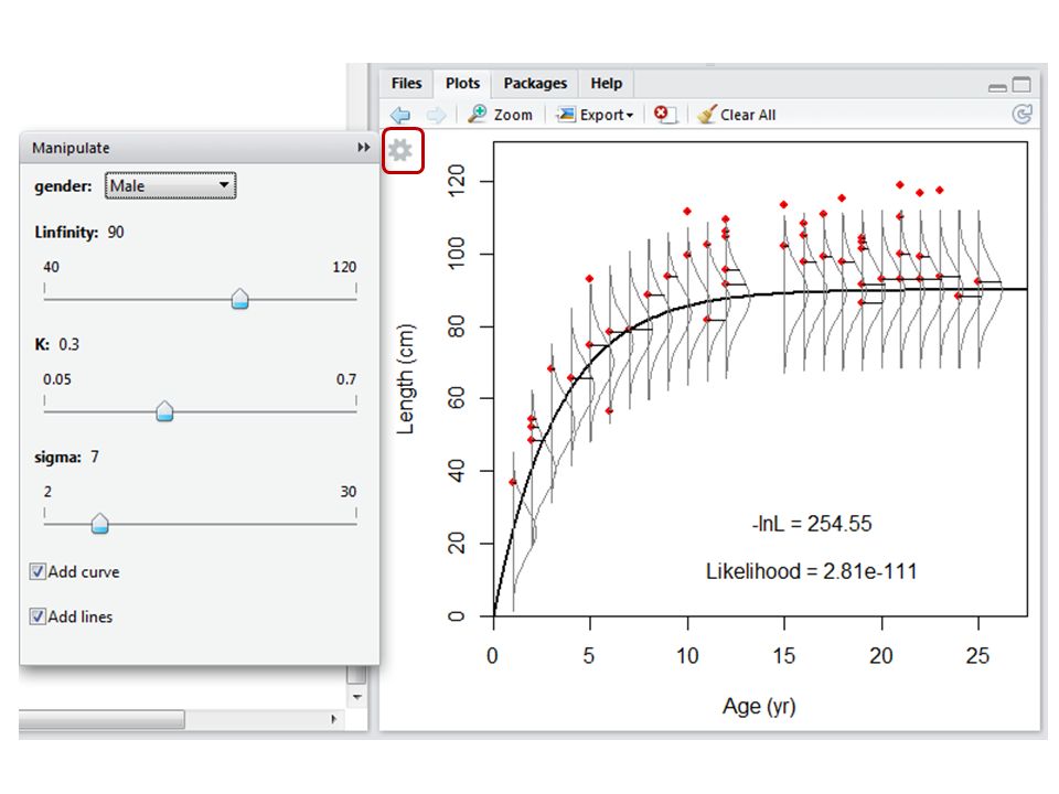
28. How I used manipulate() VB.like.sliders <- function(gender, Linfinity, K, sigma, add.curve, add.lines) { #make plot, calculate NLL, report NLL } manipulate(VB.like.sliders(gender, Linfinity, K, sigma, add.curve, add.lines), gender = picker("Male","Female"), Linfinity = slider(min=40, max=120, initial=90, step=0.001), K = slider(min=0.05, max=0.7, initial=0.3, step=0.001), sigma = slider(min=2, max=30, initial=7, step=0.001), add.curve = checkbox(TRUE, "Add curve"), add.lines = checkbox(TRUE, "Add lines"))

30. In-class exercise 2 Group class activity to find the lowest possible total negative log-likelihood (males) Use RStudio and package manipulate to run the code in "Lecture 5 manipulate.r" Play with the sliders for K, L inf, and  to find values that produce the smallest possible negative log- likelihood, -lnL tot If you find a better value, go to the board and write down the values you found for K, L inf, , and -lnL tot At home: go through the code and figure it out