1. Presented by 翁丞世 0925970510 mob5566@gmail.com

2.  View Interpolation  Layered Depth Images  Light Fields and Lumigraphs  Environment Mattes  Video-Based Rendering

4.  13.1.1 View-Dependent Texture Maps  13.1.2 Application: Photo Tourism

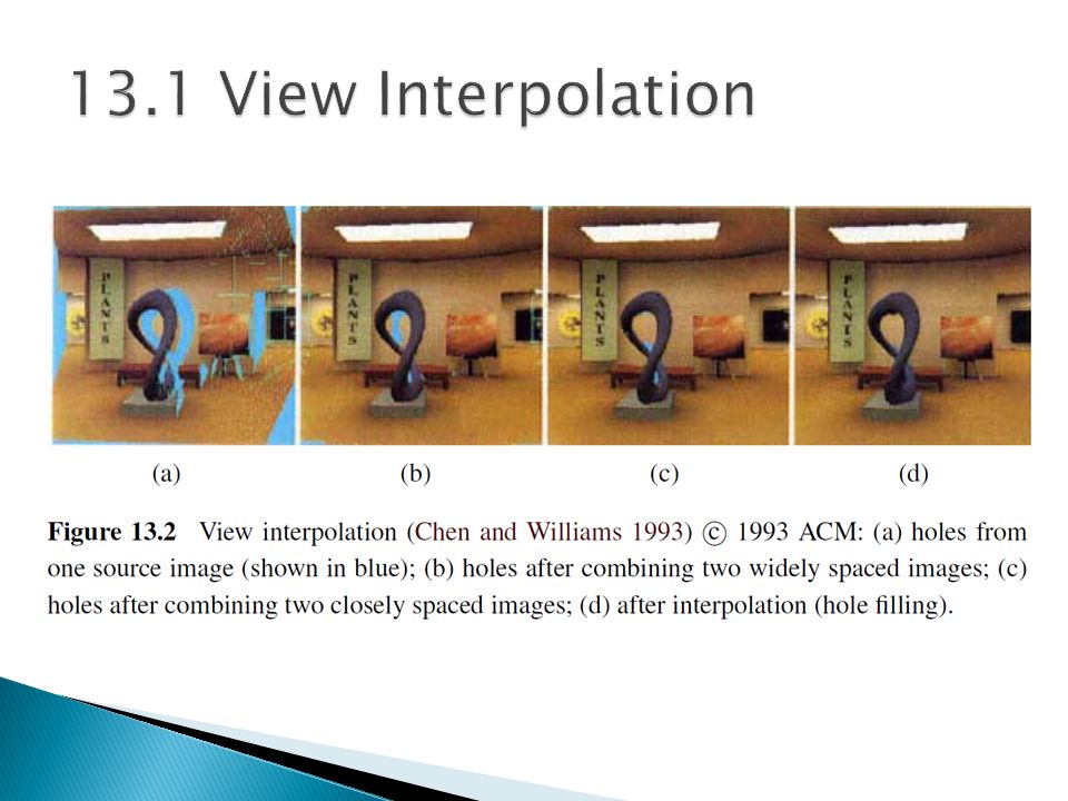
5.  View interpolation creates a seamless transition between a pair of reference images using one or more pre-computed depth maps.  Closely related to this idea are view- dependent texture maps, which blend multiple texture maps on a 3D model’s surface.

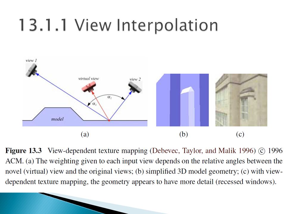
7.  View-dependent texture maps are closely related to view interpolation.  Instead of associating a separate depth map with each input image, a single 3D model is created for the scene, but different images are used as texture map sources depending on the virtual camera’s current position.

9.  Given a new virtual camera position, the similarity of this camera’s view of each polygon (or pixel) is compared with that of potential source images.  The images are then blended using a weighting that is inversely proportional to the angles between the virtual view and the source views (Figure 13.3a).

10.  Even though the geometric model can be fairly coarse, blending between different views gives a strong sense of more detailed geometry because of the parallax (visual motion) between corresponding pixels.

12.  13.2.1 Imposters, Sprites, and Layers

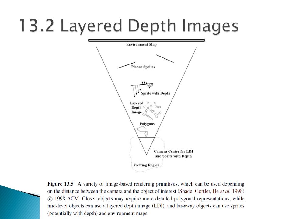
13.  When a depth map is warped to a novel view, holes and cracks inevitably appear behind the foreground objects.  One way to alleviate this problem is to keep several depth and color values (depth pixels) at every pixel in a reference image (or, at least for pixels near foreground–background transitions) (Figure 13.5).

14.  The resulting data structure, which is called a Layered Depth Image (LDI), can be used to render new views using a back-to-front forward warping algorithm (Shade, Gortler, He et al. 1998).

16.  An alternative to keeping lists of color-depth values at each pixel, as is done in the LDI, is to organize objects into different layers or sprites.

18.  13.3.1 Unstructured Lumigraph  13.3.2 Surfaces Light Fields  13.3.3 Applications: Concentric Mosaics

19.  Is it possible to capture and render the appearance of a scene from all possible viewpoints and, if so, what is the complexity of the resulting structure?  Let us assume that we are looking at a static scene, i.e., one where the objects and illuminants are fixed, and only the observer is moving around.

20.  We can describe each image by the location and orientation of the virtual camera (6 DOF).  If we capture a two-dimensional spherical image around each possible camera location, we can re-render any view from this information. DOF: Degree Of Freedom

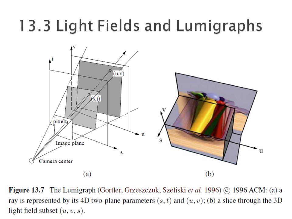
21.  To make the parameterization of this 4D function simpler, let us put two planes in the 3D scene roughly bounding the area of interest, as shown in Figure 13.7a.  Any light ray terminating at a camera that lives in front of the st plane (assuming that this space is empty) passes through the two planes at (s, t) and (u, v) and can be described by its 4D coordinate (s, t, u, v).

23.  This diagram (and parameterization) can be interpreted as describing a family of cameras living on the st plane with their image planes being the uv plane.  The uv plane can be placed at infinity, which corresponds to all the virtual cameras looking in the same direction.

24.  While a light field can be used to render a complex 3D scene from novel viewpoints, a much better rendering (with less ghosting) can be obtained if something is known about its 3D geometry.  The Lumigraph system of Gortler, Grzeszczuk, Szeliski et al. (1996) extends the basic light field rendering approach by taking into account the 3D location of surface points corresponding to each 3D ray.

25.  While a light field can be used to render a complex 3D scene from novel viewpoints, a much better rendering (with less ghosting) can be obtained if something is known about its 3D geometry.  The Lumigraph system of Gortler, Grzeszczuk, Szeliski et al. (1996) extends the basic light field rendering approach by taking into account the 3D location of surface points corresponding to each 3D ray.

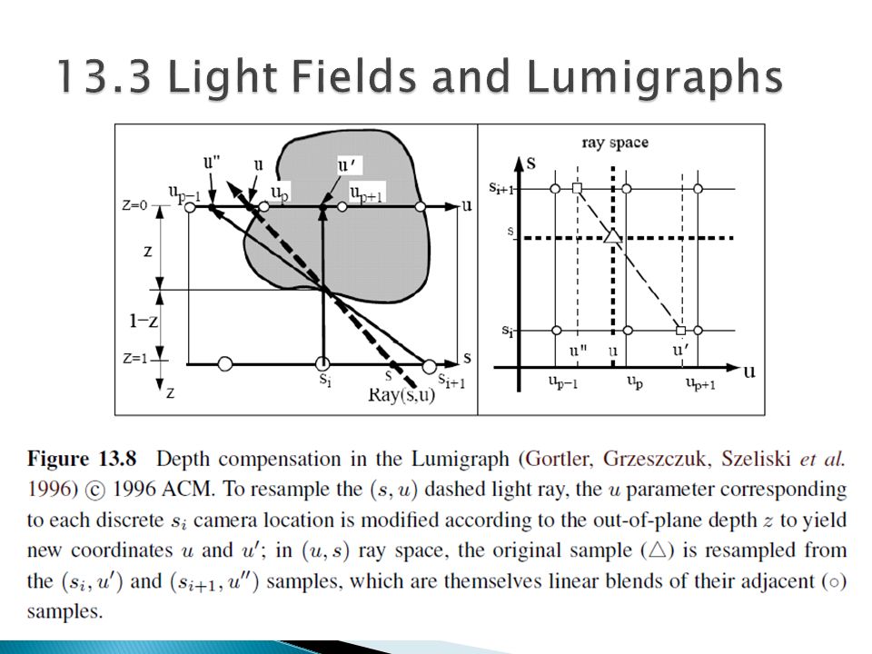
26.  Consider the ray (s, u ) corresponding to the dashed line in Figure 13.8, which intersects the object’s surface at a distance z from the uv plane.  Instead of using quadri-linear interpolation of the nearest sampled (s, t, u, v ) values around a given ray to determine its color, the (u, v ) values are modified for each discrete (si, ti ) camera.

28.  When the images in a Lumigraph are acquired in an unstructured (irregular) manner, it can be counterproductive to resample the resulting light rays into a regularly binned (s, t, u, v ) data structure.  This is both because resampling always introduces a certain amount of aliasing and because the resulting gridded light field can be populated very sparsely or irregularly.

29.  The alternative is to render directly from the acquired images, by finding for each light ray in a virtual camera the closest pixels in the original images.  The unstructured Lumigraph rendering (ULR) system of Buehler, Bosse, McMillan et al. (2001) describes how to select such pixels by combining a number of fidelity criteria, including epipole consistency (distance of rays to a source camera’s center), angular deviation (similar incidence direction on the surface), resolution (similar sampling density along the surface), continuity (to nearby pixels), and consistency (along the ray).

30.  If we know the 3D shape of the object or scene whose light field is being modeled, we can effectively compress the field because nearby rays emanating from nearby surface elements have similar color values.

31.  These observations underlie the surface light field representation introduced by Wood, Azuma, Aldinger et al. (2000).  In their system, an accurate 3D model is built of the object being represented.

32.  The Lumisphere of all rays emanating from each surface point is estimated or captured (Figure 13.9).  Nearby Lumispheres will be highly correlated and hence amenable to both compression and manipulation.