1. Stars and magnetic activity
Heidi Korhonen
Astrophysikalisches Institut Potsdam

2. Outline Stars General properties Rotation Stellar activity Solar
Light curve inversions
Doppler imaging
Principle
Requirements
Results

3. Spectral classification 1 Morgan-Keenan spectral classification
Colour M R L
Spectral lines O K
Blue 60 15
Ionized atoms, especially helium B K
Blue-white 18 7
20 000
Neutral helium, some hydrogren A K
White
3.2
2.3 80
Strong hydrogen, some ionized metals F K
Yellow-white
1.7
1.3 6
Hydrogen and ionized metals, such as calcium and iron G K
Yellow
1.0
Ionized calcium and both neutral and ionized metals K K
Orange
0.9
0.4
Neutral metals K
Red
0.04
Strong molecules, e.g., titanium oxide and some neutral calcium
EARLY
---
LATE

4. Spectral classification 2

5. Luminosity class 1
A number of different luminosity classes are distinguished:
Ia most luminous supergiants
Ib less luminous supergiants;
II bright giants
III normal giants
IV subgiants
V main sequence stars (dwarfs)

6. Luminosity class 2

7. Internal structure of the Sun
Other stars have different configurations in their interiors

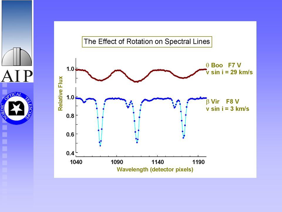
8. Stellar rotation Main sequence:
Early-type stars (O, B and A) have large rotational velocities, typically between 100 and 200 km/sec
At spectral type F, there is a rapid decline from about 100 km/sec at F0 to 10 km/sec at G0.
The Sun (G2) rotates at about 2 km/sec
Reder stars have usually rorational velocity of 1 km/sec and slower
At ZAMS all stars rotate rapidly, but the late type stars brake fast during the first ~ tens of millions of years
At main sequence cool stars enter a weak braking face that lasts billions of years

10. -dynamo
The -effect
SOHO
Solar magnetic field is generated by a magnetic dynamo within the Sun
In the -effect the fields are stretched out and wound around the Sun by differential rotation
Twisting of the magnetic filed lines is caused by the effects of the Sun‘s rotation, so called -effect

11. Magnetic activity
SOHO

12. Solar photosphere
SST

13. Solar cycle
Solar activity has on average 11 year cycle, with polarity change 22 years
First spots of the new cycle at latitude 30-35, last spots of the cycle within 10 of the equator  butterfly diagram

14. Solar chromosphere
NOAA/SEL/USAF

15. Flares
SOHO

16. Solar corona
SOHO

17. Stellar photosphere
Long-term V band photometry of FK Com (Korhonen et al. 2001)
Phased light-curves for and results
from light-curve inversions
Korhonen et al. 2002

18. Stellar chromosphere Observed for example with: H Ca II H&K
Mg II h & k
certain ion lines
Most famous study of stellar chromospheres is the Mt. Wilson HK survey
Started by Olin Wilson in mid 1960‘s
Has monitored hundred stars continuosly since then
In total more than 400 stars monitored, both dwarfs and giants

19. HK Survey 1
If we place the slit of a spectrograph across the surface of the Sun, we can trace the change in the emission of the calcium K line.
The size and extent of chromospheric active regions on the Sun varies dramatically over the course of the activity cycle.

20. HK Survey 2 HD 16160 Spectral type K3V Cycle length 13.2 yrs HD 101501
Spectral type G8V
No cycles, but variability
HD 9562
Spectral type G2V
Flat

21. Stellar corona Surface fields from the Zeeman-Doppler imaging maps
Coronal fields extrapolated from the surface fields
Here example for AB Dor:
ZDI Donati et al
Coronal extrapolation Jardine et al

22. Light-curve inversions

23. Doppler imaging
In Doppler imaging the distortions appearing in the observed line profile due to the presence of spots and moving due to the stellar rotation
Ill-posed inversion problem
Many methods for solving: aximum Entropy Method (e.g., Vogt et al 1987 ), Tikhonov Regularization (e.g., Piskunov et al 1990), Occamian Approach (Berdyugina 1998), Principal Components Analysis (Savanov & Strassmeier 2005)
From Svetlana Berdyugina

24. Requirements Instrumentation High spectral resolution
High signal-to-noise ratio
Object
Good phase coverage (convenient rotation period)
Rapid rotation
Not too long exposure time (bright)
Something to map!

25. vsini Simulations by Silva Järvinen Vsini = 45 km/s Vsini = 30 km/s
Resolution:
S/N: infinite
Phases: 20

26. Phase smearing
During the observations the star rotates and the bump moves in the lineprofile
The bump signal will be smeared
Integration time should be as short as possible:
t0.01Prot
Examples:
Prot = 20 days t > 4.5 hours
Prot = 5 days t  70 minutes
Prot = 2 days t  30 minutes
Prot = 0.5 days t  7 minutes

27. Results FK Com: Korhonen et al 2004 II Peg: Berdyugina et al 1998
² CrB: Strassmeier & Rice 2003