Download presentation
Presentation is loading. Please wait.

2
In order to produce a good, every firms uses various inputs. The amount spent on these inputs is called cost of production. These factors are to be compensated by the firm for their contribution in producing the commodity. This compensation of (factor price) is the cost.
 is the cost..")
3
Money Cost Real Cost Accounting Cost Opportunity Cost Economic Cost Social Cost Explicit Cost and Implicit Cost Fixed and Variable Costs

4
An input is valuable because it is scarce or limited If we use the input to produce one good, it is not available for producing something else The opportunity cost is the cost of next best alternative forgone. It is also called alternative cost Suppose a farmer can grow wheat as well as rice on a piece of land. He grows wheat and forgoes (sacrifices) the production of rice. If the price of rice, that he forgoes is Rs 1,000, then the opportunity cost of growing wheat is Rs 1000.
 the production of rice. If the price of rice, that he forgoes is Rs 1,000, then the opportunity cost of growing wheat is Rs")
5
The alternative or opportunity cost of producing one unit of commodity ‘X’ is the amount of commodity ‘Y’ that must be sacrificed in order to use resources to produce ‘X’ rather than ‘Y’ Suppose by using some set of inputs a firm can produce 6 units of X or 12 units of Y 6X = 12 Y, Or the opportunity cost of 1 unit of’ X’ in terms of ‘Y’ 12/6 = 2Y

6
This means that, Same amount of inputs can be used to produce 1unit of ‘X’ or 2 units of ‘Y’ To produce 1unit of ‘X’, the firm has to sacrifice the production of 2 units of ‘Y’ Thus opportunity cost of 1 unit of ‘X’ is 2 units of ‘Y’

7
In the short run at least one or some factors (inputs) are fixed and some are variable Generally the firm’s plant, manufacturing facilities, equipment and machinery are held to be fixed as they cannot be changed easily in a short period of time. The scale f production or plant capacity is fixed. However output can be changed by changing the amount of variable inputs like labour, raw material, power etc.

8
Long run is that time period in which all factor inputs are variable. New plants can be set up, existing ones can be shut down, new machinery can be installed and old ones can be replaced etc. Therefore it is possible to change all the factors of production.

9
TOTAL COST TOTAL FIXED COST TOTAL VARIABLE COST AVERAGE COST AVERAGE FIXED COST AVERAGE VARIABLE COST MARGINAL COST (always variable in nature)
")
10
Fixed Payments of rent for building. Interest on capital. Insurance premium Depreciation Property and business taxes, license fees etc. Variable Prices of raw materials, Wages paid for labour Fuel and power sales tax Freight (or transportation) charges..
 charges...")
11
TC = TFC + TVC Total cost (TC) is the sum of total fixed cost and the total variable cost for each level of output. Total cost always rises with rise in output. To get more output, the firm needs more inputs and therefore costs will be more Cost of fixed inputs is called total fixed costs. This type of cost does not change with the change in output. TFC = Units of Fixed Factors * Price of the Factor

12
Qty of Output Fixed Cost (Rs) 050 1 2 3 4 5 6 output
 output")
13
Qty of Output Variable Cost (Rs) 00 110 218 324 428 532 638
")
14
OutputFixed Cost (Rs)Variable Cost (Rs) Total Cost (Rs) 0100 1 20 2101828 3102434 4102838 5103242 6103848 7104656 8106272 TOTAL COST
Variable Cost (Rs) Total Cost (Rs) TOTAL COST")
15
Increasing returns to factor causes more than proportionate increase in output and cost increases at a decreasing rate (stage 1) Constant returns to factor causes the same proportionate increase in output and cost increases at a constant rate (stage 2) Diminishing returns to factor causes less than proportionate increase in output and cost increases at an increasing rate (stage 3)
 Constant returns to factor causes the same proportionate increase in output and cost increases at a constant rate (stage 2) Diminishing returns to factor causes less than proportionate increase in output and cost increases at an increasing rate (stage 3)")
17
TVC,TC is always increasing with the increase in output: First at a decreasing rate Then at an increasing rate TFC is always fixed and never increases or decreases in the short run.

18
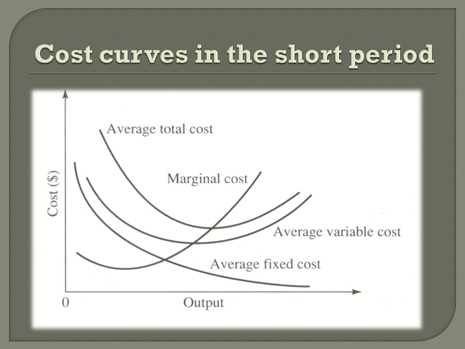
Average cost is the cost per unit of output. Average Fixed Cost Average Variable Cost Average Total Cost or (average cost) Average Fixed Cost = TFC / Q, where Q is the quantity of output
 Average Fixed Cost = TFC / Q, where Q is the quantity of output.")
19
OutputFixed cost AFC 110 2 5 3 3.3 4102.5 5102 6 1.7 7101.4

20
AFC is continuously declining curve as total output increases It never touches X axis as fixed cost can never be zero Average variable cost It is the per unit variable cost AVC = TVC / Q

21
OutputTVCAVC 110 2189 3248 4287 5326.4 6386.3 7466.6

22
It is clear from the figure that AVC has been falling in the initial stages of production because of increasing returns of the variable factor. This causes the cost to diminish But after a point, law of diminishing returns starts operating and thus variable costs start increasing. AVC is U shaped curve because of Law of Variable Proportions

23
AC = TC / Q = AFC + AVC OUTPUTAFC (Rs)AVC (Rs)AC = AVC +AFC 110 20 25914 33.3811.3 42.579.5 526.48.4 61.76.38 71.46.68 81.27.89
AVC (Rs)AC = AVC +AFC")
25
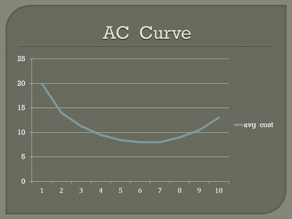
1.AC is a combination of AFC and AVC. In the initial stages AFC and AVC both are falling, and thus AC is also falling. When AC reaches the minimum point, optimum level of output is achieved Optimum level of output is that output at which per unit cost of production is lowest Beyond this optimum point, AVC will start rising

26
2. Application of Law of Variable Proportions U shaped curve is because of returns to factor in the short run In the short run, production is according to Law of Increasing returns or diminishing costs (stage 1) Constant returns or Constant Costs (stage 2) Diminishing returns or increasing costs (stage 3)
 Constant returns or Constant Costs (stage 2) Diminishing returns or increasing costs (stage 3).")
27
Marginal cost is the increase in total cost when output is increased by one unit. Suppose the total cost of producing 10 units is Rs 150. When 11 units are produced the cost goes up to Rs 200 Therefore MC = Rs 150 – Rs 200 = Rs 50 MC = TC = TC n – TC n-1 Output

28
MC is dependent on variable costs and not fixed costs because fixed cost does not change with increase in output. Units of OutputTotal Cost (Rs)Marginal Cost (Rs) 12020 – 0 = 20 22828 – 20 = 8 33434 – 28 = 6 43838 – 34 = 4 54242 – 38 = 4 64848 – 42 = 6 75656 – 48 = 8 87272 – 56 = 16
Marginal Cost (Rs) – 0 = – 20 = – 28 = – 34 = – 38 = – 42 = – 48 = – 56 = 16.")
30
In the initial stage when output increases, TC and VC increase at diminishing rate. It is because of increasing returns to a factor. Thus the firm enjoys several economies. Cost of every additional unit is less than earlier units. Thus MC curve falls. After some level of output, rate of increase in TC and VC is minimum. Thus MC is also minimum.

31
After a certain period of time TC and VC increase at an increasing rate because of law of diminishing returns. The firm suffers several diseconomies. Cost of each additional unit is more than the previous units. Thus MC curve starts rising and assumes a U shape.

32
OutputTCFCVCACMC 12010 20 2281018148 334102411.36 43810289.54 54210328.44 648103886 756104688 8721062916

33
AC and MC curves MC AC COST OUTPUT P L Q B C O

34
When AC falls, MC is less than AC When AC rises, MC is greater than AC MC cuts AC at its lowest point, MC is equal to AC when AC is minimum.

36
Output (Q) Costs (£) AFC AVC MC x AC z y
 Costs (£) AFC AVC MC x AC z y")
37
As long as MP is rising MC is falling. When MP is maximum, MC is minimum As long as AP is rising, AC is falling. When AP is maximum, AC is minimum. MP intersects AP at its maximum point MC intersects AC at its minimum point

38
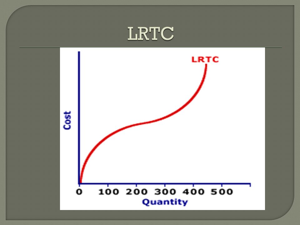
Long run Total Cost Long run Average Cost Long run Marginal Cost Long run Total cost (LTC) In the long run all the costs are variable costs. The long run total cost is the least possible cost of producing any given level of output when all inputs are variable.

39
LTC < STC In the long run the firm can attain min cost because they can select optimal plant size or least cost factor proportion

41
LAC is that curve which shows the minimum cost per unit of producing each output level, corresponding to different scales of productivity LAC = LTC/ OUTPUT Different plants are possible in the long run because of different demand for output. Each plant will have its own SAC

42
LAC is a combination of different SACs of different plants LAC is tangent to each SAC curve at some point The point of optimum utilization is the point at which lowest point of SAC coincides at lowest point of LAC

44
SRAC 3 Costs Output O SRAC 4 SRAC 5 5 factories 4 factories 3 factories 2 factories 1 factory SRAC 1 SRAC 2

45
SRAC 1 SRAC 3 SRAC 2 SRAC 4 SRAC 5 LRAC Costs Output O

46
Costs Output O Examples of short-run average cost curves

47
LRAC Costs Output O

48
Economies of Scale 1. Division and specialization of labour 2. Technical economies 3. Economies of indivisibility Diseconomies of scale Returns to Scale

49
Output O Costs LRAC Economies of scale Constant costs Diseconomies of scale

50
It is the addition to the total cost due to production of one extra unit of output when the quantity of all the inputs are changed. Optimum level of output is that output at which LAC is equal to SAC. If the output is less than the optimum level, SMC will be less than LMC. If the output is more than the optimum level, SMC will be more than LMC.

Similar presentations