Download presentation
Presentation is loading. Please wait.

1
Cornea Data Main Point: OODA Beyond FDA Recall Interplay: Object Space Descriptor Space

2
Robust PCA What is multivariate median? There are several! ( “ median ” generalizes in different ways) i.Coordinate-wise median Often worst Not rotation invariant (2-d data uniform on “ L ” ) Can lie on convex hull of data (same example) Thus poor notion of “ center ”
 i.Coordinate-wise median Often worst Not rotation invariant (2-d data uniform on L ) Can lie on convex hull of data (same example) Thus poor notion of center .")
3
Robust PCA

4
M-estimate (cont.): “ Slide sphere around until mean (of projected data) is at center ”
: Slide sphere around until mean (of projected data) is at center")
5
Robust PCA Robust PCA 3: Spherical PCA Idea: use “ projection to sphere ” idea from M-estimation In particular project data to centered sphere “ Hot Dog ” of data becomes “ Ice Caps ” Easily found by PCA (on proj ’ d data) Outliers pulled in to reduce influence Radius of sphere unimportant
 Outliers pulled in to reduce influence Radius of sphere unimportant")
6
Robust PCA Spherical PCA for Toy Example: Curve Data With an Outlier First recall Conventional PCA

7
Robust PCA Spherical PCA for Toy Example: Now do Spherical PCA Better result?

8
Robust PCA Rescale Coords Unscale Coords Spherical PCA

9
Robust PCA Elliptical PCA for cornea data: Original PC2, Elliptical PC2

10
Big Picture View of PCA Alternate Viewpoint: Gaussian Likelihood When data are multivariate Gaussian PCA finds major axes of ellipt ’ al contours of Probability Density Maximum Likelihood Estimate Mistaken idea: PCA only useful for Gaussian data

11
Big Picture View of PCA Raw Cornea Data: Data – Median (Data – Median) ------------------- MAD
 MAD")
12
Big Picture View of PCA Check for Gaussian dist ’ n: Stand ’ zed Parallel Coord. Plot E.g. Cornea data (recall image view of data) Several data points > 20 “ s.d.s ” from the center Distribution clearly not Gaussian Strong kurtosis ( “ heavy tailed ” ) But PCA still gave strong insights
 Several data points > 20 s.d.s from the center Distribution clearly not Gaussian Strong kurtosis ( heavy tailed ) But PCA still gave strong insights.")
13
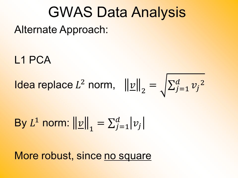
GWAS Data Analysis

14
Genome Wide Association Study (GWAS) Cystic Fibrosis Study: Wright et al (2011) Interesting Feature: Some Subjects are Close Relatives (e.g. ~half SNPs are same)
.")
15
GWAS Data Analysis PCA View Clear Ethnic Groups And Several Outliers! Eliminate With Spherical PCA?

16
GWAS Data Analysis Spherical PCA Looks Same?!? What is going on?

17
GWAS Data Analysis

19
L1 PCA Challenge: L1 Projections Hard to Interpret 2-d Toy Example Note Outlier

20
L1 PCA Conventional L2 PCA Outlier Pulls Off PC1 Direction

21
L1 PCA Much Better PC1 Direction

22
L1 PCA Much Better PC1 Direction But Very Strange Projections (i.e. Little Data Insight)
")
23
L1 PCA Reason: SVD Rotation Before L1 Computation Note: L1 Methods Not Rotation Invariant

24
L1 PCA Challenge: L1 Projections Hard to Interpret (i.e. Little Data Insight) Solution: 1)Compute PC Directions Using L1 2)Compute Projections (Scores) Using L2 Called “Visual L1 PCA” (VL1PCA) Recent work with Yihui Zhou
 Solution: 1)Compute PC Directions Using L1 2)Compute Projections (Scores) Using L2 Called Visual L1 PCA (VL1PCA) Recent work with Yihui Zhou.")
25
L1 PCA VL1 PCA Excellent PC Directions Interpretable Scores

26
VL1 PCA 10-d Toy Example: Parabolas From Before With Two Outliers

27
VL1 PCA 10-d Toy Example: L2PCA Strongly Impacted (In All Components)
")
28
VL1 PCA 10-d Toy Example: SCPA & VL1PCA Nicely Robust (Vl1PCA Slightly Better)
")
29
VL1 PCA 10-d Toy Example: L1PCA Hard To Interpret

30
GWAS Data L1 PCA No Longer Feels Outliers But Still Highlights Individuals

31
GWAS Data VL1 PCA Best Focus On Ethnic Groups

32
GWAS Data VL1 PCA Best Focus On Ethnic Groups Seems To Find Unlabelled Clusters

33
Detailed Look at PCA Now Study “Folklore” More Carefully BackGround History Underpinnings (Mathematical & Computational) Good Overall Reference: Jolliffe (2002)
 Good Overall Reference: Jolliffe (2002)")
34
PCA: Rediscovery – Renaming Statistics: Principal Component Analysis (PCA) Social Sciences: Factor Analysis (PCA is a subset) Probability / Electrical Eng: Karhunen – Loeve expansion Applied Mathematics: Proper Orthogonal Decomposition (POD) Geo-Sciences: Empirical Orthogonal Functions (EOF)
 Social Sciences: Factor Analysis (PCA is a subset) Probability / Electrical Eng: Karhunen – Loeve expansion Applied Mathematics: Proper Orthogonal Decomposition (POD) Geo-Sciences: Empirical Orthogonal Functions (EOF)")
35
An Interesting Historical Note The 1 st (?) application of PCA to Functional Data Analysis: Rao (1958) 1 st Paper with “Curves as Data Objects” viewpoint
 application of PCA to Functional Data Analysis: Rao (1958) 1 st Paper with Curves as Data Objects viewpoint")
36
Detailed Look at PCA Three Important (& Interesting) Viewpoints: 1. Mathematics 2. Numerics 3. Statistics Goal: Study Interrelationships

37
Detailed Look at PCA Three Important (& Interesting) Viewpoints: 1. Mathematics 2. Numerics 3. Statistics 1 st : Review Linear Alg. and Multivar. Prob.

38
Review of Linear Algebra

39
Review of Linear Algebra (Cont.) SVD Full Representation: = Graphics Display Assumes
 SVD Full Representation: = Graphics Display Assumes")
40
Review of Linear Algebra (Cont.) SVD Full Representation: = Full Rank Basis Matrix
 SVD Full Representation: = Full Rank Basis Matrix")
41
Review of Linear Algebra (Cont.) SVD Full Representation: = Full Rank Basis Matrix All 0s in Bottom (and off diagonal)
 SVD Full Representation: = Full Rank Basis Matrix All 0s in Bottom (and off diagonal)")
42
Review of Linear Algebra (Cont.) SVD Reduced Representation: = These Columns Get 0ed Out
 SVD Reduced Representation: = These Columns Get 0ed Out")
43
Review of Linear Algebra (Cont.) SVD Reduced Representation: =
 SVD Reduced Representation: =")
44
Review of Linear Algebra (Cont.) SVD Reduced Representation: = Also, Some of These May be 0
 SVD Reduced Representation: = Also, Some of These May be 0")
45
Review of Linear Algebra (Cont.) SVD Compact Representation: =
 SVD Compact Representation: =")
46
Review of Linear Algebra (Cont.) SVD Compact Representation: = These Get 0ed Out
 SVD Compact Representation: = These Get 0ed Out")
47
Review of Linear Algebra (Cont.) SVD Compact Representation: =
 SVD Compact Representation: =")
48
Review of Linear Algebra (Cont.)
")
58
Recall Linear Algebra (Cont.) Moore-Penrose Generalized Inverse: For
 Moore-Penrose Generalized Inverse: For")
59
Recall Linear Algebra (Cont.) Easy to see this satisfies the definition of Generalized (Pseudo) Inverse symmetric
 Easy to see this satisfies the definition of Generalized (Pseudo) Inverse symmetric")
60
Recall Linear Algebra (Cont.)
")
62
Recall Multivar. Prob.

63
Outer Product Representation:, Where:

64
Recall Multivar. Prob.

65
PCA as an Optimization Problem Find Direction of Greatest Variability:

66
PCA as an Optimization Problem Find Direction of Greatest Variability:

67
PCA as an Optimization Problem Find Direction of Greatest Variability: Raw Data

68
PCA as an Optimization Problem Find Direction of Greatest Variability: Mean Residuals (Shift to Origin)
")
69
PCA as an Optimization Problem Find Direction of Greatest Variability: Mean Residuals (Shift to Origin)
")
70
PCA as an Optimization Problem Find Direction of Greatest Variability: Centered Data

71
PCA as an Optimization Problem Find Direction of Greatest Variability: Centered Data Projections

72
PCA as an Optimization Problem Find Direction of Greatest Variability: Centered Data Projections Direction Vector

73
PCA as Optimization (Cont.) Find Direction of Greatest Variability: Given a Direction Vector, (i.e. ) (Variable, Over Which Will Optimize)
 (Variable, Over Which Will Optimize).")
74
PCA as Optimization (Cont.) Find Direction of Greatest Variability: Given a Direction Vector, (i.e. ) Projection of in the Direction :
 Projection of in the Direction :.")
75
PCA as Optimization (Cont.) Find Direction of Greatest Variability: Given a Direction Vector, (i.e. ) Projection of in the Direction : Variability in the Direction :
 Projection of in the Direction : Variability in the Direction :.")
76
PCA as Optimization (Cont.) Find Direction of Greatest Variability: Given a Direction Vector, (i.e. ) Projection of in the Direction : Variability in the Direction :
 Projection of in the Direction : Variability in the Direction :.")
77
PCA as Optimization (Cont.) Find Direction of Greatest Variability: Given a Direction Vector, (i.e. ) Projection of in the Direction : Variability in the Direction :
 Projection of in the Direction : Variability in the Direction :.")
78
PCA as Optimization (Cont.) Variability in the Direction :
 Variability in the Direction :")
79
PCA as Optimization (Cont.) Variability in the Direction : i.e. (Proportional to) a Quadratic Form in the Covariance Matrix
 a Quadratic Form in the Covariance Matrix.")
80
PCA as Optimization (Cont.) Variability in the Direction : i.e. (Proportional to) a Quadratic Form in the Covariance Matrix Simple Solution Comes from the Eigenvalue Representation of :
 a Quadratic Form in the Covariance Matrix Simple Solution Comes from the Eigenvalue Representation of :.")
81
PCA as Optimization (Cont.) Variability in the Direction : i.e. (Proportional to) a Quadratic Form in the Covariance Matrix Simple Solution Comes from the Eigenvalue Representation of : Where is Orthonormal, &
 a Quadratic Form in the Covariance Matrix Simple Solution Comes from the Eigenvalue Representation of : Where is Orthonormal, &.")
82
PCA as Optimization (Cont.) Variability in the Direction :
 Variability in the Direction :")
83
PCA as Optimization (Cont.) Variability in the Direction : But
 Variability in the Direction : But")
84
PCA as Optimization (Cont.) Variability in the Direction : But = “ Transform of ”
 Variability in the Direction : But = Transform of")
85
PCA as Optimization (Cont.) Variability in the Direction : But = “ Transform of ” = “ Rotated into Coordinates”,
 Variability in the Direction : But = Transform of = Rotated into Coordinates ,")
86
PCA as Optimization (Cont.) Variability in the Direction : But = “ Transform of ” = “ Rotated into Coordinates”, and the Diagonalized Quadratic Form Becomes
 Variability in the Direction : But = Transform of = Rotated into Coordinates , and the Diagonalized Quadratic Form Becomes")
87
PCA as Optimization (Cont.) Now since is an Orthonormal Basis Matrix, and
 Now since is an Orthonormal Basis Matrix, and")
88
PCA as Optimization (Cont.) Now since is an Orthonormal Basis Matrix, and So the Rotation Gives a Distribution of the Energy of Over the Eigen-Directions
 Now since is an Orthonormal Basis Matrix, and So the Rotation Gives a Distribution of the Energy of Over the Eigen-Directions")
89
PCA as Optimization (Cont.) Now since is an Orthonormal Basis Matrix, and So the Rotation Gives a Distribution of the Energy of Over the Eigen-Directions And is Max’d (Over ), by Putting all Energy in the “Largest Direction”, i.e., Where “Eigenvalues are Ordered”,
 Now since is an Orthonormal Basis Matrix, and So the Rotation Gives a Distribution of the Energy of Over the Eigen-Directions And is Max’d (Over ), by Putting all Energy in the Largest Direction , i.e., Where Eigenvalues are Ordered ,")
90
PCA as Optimization (Cont.)
")
91
Iterated PCA Visualization

92
PCA as Optimization (Cont.)
")
93
Recall Toy Example

94
PCA as Optimization (Cont.) Recall Toy Example Empirical (Sample) EigenVectors
 Recall Toy Example Empirical (Sample) EigenVectors")
95
PCA as Optimization (Cont.) Recall Toy Example Theoretical Distribution
 Recall Toy Example Theoretical Distribution")
96
PCA as Optimization (Cont.) Recall Toy Example Theoretical Distribution & Eigenvectors
 Recall Toy Example Theoretical Distribution & Eigenvectors")
97
PCA as Optimization (Cont.) Recall Toy Example Empirical (Sample) EigenVectors Theoretical Distribution & Eigenvectors Different!
 Recall Toy Example Empirical (Sample) EigenVectors Theoretical Distribution & Eigenvectors Different!")
98
Connect Math to Graphics 2-d Toy Example From First Class Meeting Simple, Visualizable Descriptor Space 2-d Curves as Data In Object Space

99
Connect Math to Graphics 2-d Toy Example Data Points (Curves)
")
100
Connect Math to Graphics (Cont.) 2-d Toy Example
 2-d Toy Example")
101
Connect Math to Graphics (Cont.) 2-d Toy Example Residuals from Mean = Data - Mean
 2-d Toy Example Residuals from Mean = Data - Mean")
102
Connect Math to Graphics (Cont.) 2-d Toy Example
 2-d Toy Example")
103
Connect Math to Graphics (Cont.) 2-d Toy Example
 2-d Toy Example")
104
Connect Math to Graphics (Cont.) 2-d Toy Example PC1 Projections Best 1-d Approximations of Data
 2-d Toy Example PC1 Projections Best 1-d Approximations of Data")
105
Connect Math to Graphics (Cont.) 2-d Toy Example PC1 Residuals
 2-d Toy Example PC1 Residuals")
106
Connect Math to Graphics (Cont.) 2-d Toy Example
 2-d Toy Example")
107
Connect Math to Graphics (Cont.) 2-d Toy Example PC2 Projections (= PC1 Resid’s) 2 nd Best 1-d Approximations of Data
 2-d Toy Example PC2 Projections (= PC1 Resid’s) 2 nd Best 1-d Approximations of Data")
108
Connect Math to Graphics (Cont.) 2-d Toy Example PC2 Residuals = PC1 Projections
 2-d Toy Example PC2 Residuals = PC1 Projections")
109
Connect Math to Graphics (Cont.) Note for this 2-d Example: PC1 Residuals = PC2 Projections PC2 Residuals = PC1 Projections (i.e. colors common across these pics)
.")
110
PCA Redistribution of Energy

112
PCA Redist ’ n of Energy (Cont.)
")
114
Connect Math to Graphics (Cont.) 2-d Toy Example
 2-d Toy Example")
115
Connect Math to Graphics (Cont.) 2-d Toy Example
 2-d Toy Example")
116
Connect Math to Graphics (Cont.) 2-d Toy Example
 2-d Toy Example")
117
Connect Math to Graphics (Cont.) 2-d Toy Example
 2-d Toy Example")
118
Connect Math to Graphics (Cont.) 2-d Toy Example
 2-d Toy Example")
119
Connect Math to Graphics (Cont.) 2-d Toy Example
 2-d Toy Example")
120
Connect Math to Graphics (Cont.) 2-d Toy Example
 2-d Toy Example")
121
Connect Math to Graphics (Cont.) 2-d Toy Example
 2-d Toy Example")
122
Connect Math to Graphics (Cont.) 2-d Toy Example
 2-d Toy Example")
123
PCA Redist ’ n of Energy (Cont.) Have already studied this decomposition (recall curve e.g.)
 Have already studied this decomposition (recall curve e.g.)")
124
PCA Redist ’ n of Energy (Cont.) Have already studied this decomposition (recall curve e.g.) Variation (SS) due to Mean (% of total)
 Have already studied this decomposition (recall curve e.g.) Variation (SS) due to Mean (% of total)")
125
PCA Redist ’ n of Energy (Cont.) Have already studied this decomposition (recall curve e.g.) Variation (SS) due to Mean (% of total) Variation (SS) of Mean Residuals (% of total)
 Have already studied this decomposition (recall curve e.g.) Variation (SS) due to Mean (% of total) Variation (SS) of Mean Residuals (% of total)")
126
PCA Redist ’ n of Energy (Cont.) Now Decompose SS About the Mean where: Note Inner Products this time
 Now Decompose SS About the Mean where: Note Inner Products this time")
127
PCA Redist ’ n of Energy (Cont.) Now Decompose SS About the Mean where: Recall: Can Commute Matrices Inside Trace
 Now Decompose SS About the Mean where: Recall: Can Commute Matrices Inside Trace")
128
PCA Redist ’ n of Energy (Cont.) Now Decompose SS About the Mean where: Recall: Cov Matrix is Outer Product
 Now Decompose SS About the Mean where: Recall: Cov Matrix is Outer Product")
129
PCA Redist ’ n of Energy (Cont.) Now Decompose SS About the Mean where: i.e. Energy is Expressed in Trace of Cov Matrix

130
PCA Redist ’ n of Energy (Cont.) (Using Eigenvalue Decomp. Of Cov Matrix)
 (Using Eigenvalue Decomp. Of Cov Matrix)")
131
PCA Redist ’ n of Energy (Cont.) (Commute Matrices Within Trace)
 (Commute Matrices Within Trace)")
132
PCA Redist ’ n of Energy (Cont.) (Since Basis Matrix is Orthonormal)
 (Since Basis Matrix is Orthonormal)")
133
PCA Redist ’ n of Energy (Cont.) Eigenvalues Provide Atoms of SS Decompos’n
 Eigenvalues Provide Atoms of SS Decompos’n")
134
Connect Math to Graphics (Cont.) 2-d Toy Example
 2-d Toy Example")
135
Connect Math to Graphics (Cont.) 2-d Toy Example
 2-d Toy Example")
136
Connect Math to Graphics (Cont.) 2-d Toy Example
 2-d Toy Example")
137
Connect Math to Graphics (Cont.) 2-d Toy Example
 2-d Toy Example")
138
Connect Math to Graphics (Cont.) 2-d Toy Example
 2-d Toy Example")
139
Connect Math to Graphics (Cont.) 2-d Toy Example
 2-d Toy Example")
140
PCA Redist ’ n of Energy (Cont.) Eigenvalues Provide Atoms of SS Decompos’n
 Eigenvalues Provide Atoms of SS Decompos’n")
141
PCA Redist ’ n of Energy (Cont.) Eigenvalues Provide Atoms of SS Decompos’n Useful Plots are: Power Spectrum: vs.
 Eigenvalues Provide Atoms of SS Decompos’n Useful Plots are: Power Spectrum: vs.")
142
PCA Redist ’ n of Energy (Cont.) Eigenvalues Provide Atoms of SS Decompos’n Useful Plots are: Power Spectrum: vs. log Power Spectrum: vs. (Very Useful When Are Orders of Mag. Apart)
.")
143
PCA Redist ’ n of Energy (Cont.) Eigenvalues Provide Atoms of SS Decompos’n Useful Plots are: Power Spectrum: vs. log Power Spectrum: vs. Cumulative Power Spectrum: vs.

144
PCA Redist ’ n of Energy (Cont.) Eigenvalues Provide Atoms of SS Decompos’n Useful Plots are: Power Spectrum: vs. log Power Spectrum: vs. Cumulative Power Spectrum: vs. Note PCA Gives SS’s for Free (As Eigenval’s), But Watch Factors of
, But Watch Factors of.")
145
PCA Redist ’ n of Energy (Cont.) Note, have already considered some of these Useful Plots:
 Note, have already considered some of these Useful Plots:")
146
PCA Redist ’ n of Energy (Cont.) Note, have already considered some of these Useful Plots: Power Spectrum
 Note, have already considered some of these Useful Plots: Power Spectrum")
147
PCA Redist ’ n of Energy (Cont.) Note, have already considered some of these Useful Plots: Power Spectrum Cumulative Power Spectrum
 Note, have already considered some of these Useful Plots: Power Spectrum Cumulative Power Spectrum")
148
PCA Redist ’ n of Energy (Cont.) Note, have already considered some of these Useful Plots: Power Spectrum Cumulative Power Spectrum Common Terminology: Power Spectrum is Called “Scree Plot” Kruskal (1964) Cattell (1966) (all but name “scree”) (1 st Appearance of name???)
 Note, have already considered some of these Useful Plots: Power Spectrum Cumulative Power Spectrum Common Terminology: Power Spectrum is Called Scree Plot Kruskal (1964) Cattell (1966) (all but name scree ) (1 st Appearance of name )")
149
Participant Presentation Anna Zhao Surviving in the NBA

Similar presentations


 is a technique that is useful for the compression and classification.>")

 Are You ENRolled? Tentative Title (???? Is OK) When: Next Week, Early, Oct.,>")

>")

>")


 Purpose of PCA Covariance and correlation matrices PCA using eigenvalues PCA using singular value decompositions Selection.>")

 Cogsci 108F Linear.>")

