1. SKEE 3143 Control Systems Design Chapter 2 – PID Controllers Design
Dr. Shahdan Bin Sudin
Faculty of Electrical Engineering, UTM
Room location: P08-328

2. Chapter Outline 2.1 Introduction and Re-visit
2.2 Design with Gain Adjustment
2.3 Improving the Steady State Error
2.3.1 Proportional Integral Controller (PI)
2.4 Improving the Transient Response
2.4.1 Proportional Derivative Controller (PD)
2.5 Improving Transient Response and Steady-State Error
2.5.1 Proportional-Integral-Derivative Controller (PID)
2.6 Tuning the PID using Ziegler-Nichols Technique
2.7 Controller design using MATLAB 2

3. Introduction
Root locus (RL) is a powerful tool for design of control systems.
We will study four design techniques:
Gain adjustment
Proportional-Integral (PI) controller
Proportional-Derivative (PD) controller
Proportional-Integral-Derivative (PID) controller

4. Re-visit: Input Signals

5. Re-visit: Poles and Zeros
Poles: roots of the denominator of a transfer function.
Zeros: roots of the numerator of a transfer function.
Poles and zeros can be mapped on an s-plane (pole: x, zero: o).
Important in control systems. 5

6. Re-visit: First Order System
Transfer function:
With a unit step input,

7. Re-visit: First Order System
Time response
Specifications:
time constant,
rise time, settling
time.

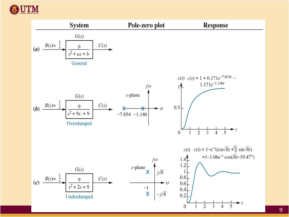
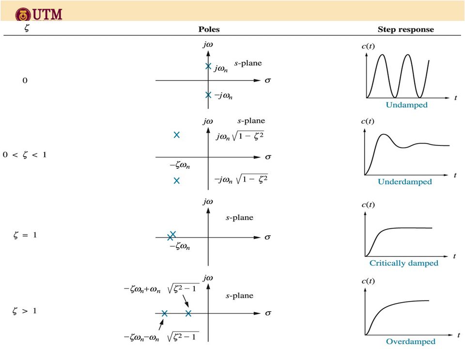
8. Revisit: Second Order System
Transfer function:
The second order system responses are determined by damping ratio,  and natural frequency, n
Time responses can be categorised into overdamped, underdamped, undamped and critically damped based on the damping ratio and pole locations.

10. 10

12. Re-visit: 2nd Order System Response
Responses:
Example

13. Re-visit: Underdamped Response
Overshoot
Rise time
Peak time
Settling time

14. Re-visit: Performance Specifications
Peak time,
Percent overshoot,
Settling time,

15. Re-visit: Additional Poles
The formulae were derived based on a purely second order system. Therefore, the formulae valid only for second order system without zero.
However, under certain conditions, a system with more that 2 poles can be approximated as a 2nd order system.
In this case, the complex poles are known as dominant poles.

16. Re-visit: Additional Poles
Consider 3 cases:
Case III behaves
as a 2nd order
response
Approximation is
valid if the third
pole more than
5 times farther to
the left
p1 and p2 are
dominant poles.
Dominant pole

17. Additional Zeros
The zeros affect the amplitude of response but do not affect the nature of the response.
Consider a 2nd order system with poles, s1,2 = -1  j Adding zero at -3, -5 and -10.
The closer the zero to the
dominant poles, the
greater the effect on
the transient response

18. Additional Zeros
Adding a positive zero,
Example
Non-minimum phase

19. Re-visit: Steady-State Errors
Steady-state error (ess) is the difference between the input and output for a prescribed test input as t  .
ess

20. Steady-State Errors
ess can be calculated using the final value theorem.
where E(s) = R(s) – C(s)
ess depends on the input and system type.
Static error constants: position constant (Kp), velocity constant (Kv) and acceleration constant (Ka).

21. 2.2 Design with Gain Adjustment

22. Second-order Approximation
The formulae for the time response specifications only valid for a pure second order system without zero.
Conditions for second order approximation:
Higher order poles are five time farther into the left that the dominant second order poles.
Closed-loop zeros are nearly cancelled by the close proximity of higher order poles. 22

23. Second-order Approximation
Figures (b) and (d) yield better approximation.
Higher order pole is farther to
the left of the dominant poles
Higher order pole cancel the closed-loop zero 23

24. Design with gain adjustment
Design procedure for higher order systems :
Sketch the root locus.
Assume the system is a second order system without zero and find the gain to meet the specifications.
Justify the second-order approximation by finding higher order poles. 24

25. Example 1
Given a unity feedback system that has the forward-path transfer function
Sketch the root locus
Design the value of K to yield 10% OS
Estimate the settling time, peak time and steady-state error for the value of K in (b).
Determine the validity of your second-order approximation. 25

26. Solution 1 K = 45.55 Ts = 1.97 s, Tp = 1.13 s, ess=0.51
Second order approximation is not valid. 26

27. Design with gain adjustment
The root locus allows us to choose a proper gain to meet a transient response specification.
As the gain is varied, we move through different regions of response.
However, we are limited to those responses that exists along the root locus only. 27

28. 2.3 Improving the Steady State Error

29. Improving the System Response
Flexibility in the design can be increased if we can design for response that are not on the root locus.
Consider the desired transient response defined by OS and settling time.
With gain adjustment, we can only obtain settling time at A to satisfy the desired OS.
Point B cannot be on the root locus with the gain adjustment.
A controller/compensator has to be designed. 29

30. Improving Steady-state Error
Compensators can also be used to improve steady-state error.
By increasing the gain, the ess reduces but OS increases.
By reducing the gain, OS reduces but ess increases.
Compensators can be designed to meet the transient response and steady-state error simultaneously. 30

31. Configurations Two configurations of compensation:
Cascade compensation: The compensation network is placed in cascade with the plant.
Feedback compensation: The compensator is placed in the feedback path
Both methods change the OL poles and zeros, thus creating a new root locus that goes through the desired CL pole location. 31

32. Proportional-Integral (PI) Controller/Compensator
PI controller/compensator is used to improve steady-state error.
ess can be improved by placing an open-loop pole at the origin as this increases the system type by one. 32

33. Proportional-Integral (PI) Controller/Compensator
Consider a system operating at a desirable response with CL pole at A.
By adding a pole to increase the system type, A is no longer a CL pole. 33

34. Proportional-Integral (PI) Controller/Compensator
To solve, a zero close to the pole at the origin has to be added. Thus A is now a CL pole.
Thus, we have improved the ess without affecting the transient response. This is known as PI controller/compensator.

35. Example 2
Given a system operating with a damping ratio of 0.174, show that the addition of the PI compensator reduces the ess to zero for a unit step input without affecting transient response.
Before compensation
After compensation 35

36. Solution 2
For a damping ratio 0.174, the dominant poles: s = ± j 3.962, K =
The third pole at and second-order approximation is valid.
Kp=8.23, ess = 36

37. Solution 2 Adding a pole at the origin and zero at -0.1.
With the same damping ratio, dominant poles, s = ± j.837, K =
Compensated CL poles and gain are approximately
the same as the
uncompensated system.
Both gives the same
transient response.
However, with PI,
system is type 1 and ess = 0. 37

38. Solution 2

39. Proportional-Integral (PI) Controller/Compensator
In general, transfer function of PI controller
Implementation 39

40. Proportional-Integral (PI) Controller/Compensator
PI controller is designed by adding a pole at the origin and a zero at s = -z.
The zero is chosen to satisfy transient response specifications.
The value of the zero can be adjusted by varying KI/KP.
If the same transient response as the uncompensated system is required, choose the zero close to the origin. Example: s = -0.1, s = 40

41. Example 3 For the unity feedback system with
design a PI controller to achieve a transient response as the following:
OS = 10 %
Settling time 16/3 s
Zero steady-state error to unit step input 41

42. Solution 3
Sketch the root locus of the system without the PI Controller.
Find the CL poles for the required transient response
Desired CL poles: s = ± j1
To achieve zero ess, add a pole at the origin.
Determine the location of the zero and let Kp = 1.
Re-sketch the root locus of the system with the PI Controller
Find the CL poles and the gain to achieve the transient and steady state responses.
 we want the overall system with the same transient response but zero steady state error. 42

43. 2.4 Improving the Transient Response

44. Proportional-Derivative (PD) Controller/Compensator
PD controller is used to improve transient response and maintaining the steady-state error.
Transient response can be improved by adding a single zero to the forward path of the feedback control system.
This zero can be represented as
A proper selection of the zero can improve the system’s transient response. 44

45. Proportional-Derivative (PD) Controller/Compensator
Zero, s = -4
Uncompensated
Zero, s = -2
Zero, s = -3

46. Proportional-Derivative (PD) Controller/Compensator
All compensated systems operate at damping ratio, 0.4 as the uncompensated system.
For all the compensated systems, the CL poles have more negative real and larger imaginary part as compared to the uncompensated system.
Thus, the compensated systems operate with shorter settling time and peak time.
System (b) gives the best transient response.
In summary, adding a zero on the forward path improves the transient response.
A proper selection of the value of the zero is required. 46

47. Proportional-Derivative (PD) Controller/Compensator47

48. Example 4
Given the system, design a PD controller to yield 16 % overshoot, with a threefold reduction in the settling time. 48

49. Solution 4
Draw the root locus without PD Controller 49

50. Solution 4 To get 16% OS, the CL poles can be found at
with Ts = 3.32 s, Tp = 1.52 s
ess = 1/Kv = 0.55 (by calculation when K = 43.35)
Third pole at s = Thus second order approximation is valid.
Desired specifications:
OS 16 %, Ts = 3.32/3 = s
Desired CL poles, (calculation)
s = ± j6.193
How to calculate?
use triangle

51. Solution 4
The zero is calculated using angle property: total angles from poles to the root – total angles from zeros to the root = 1800.
The angle =
How?
Thus, z = 3.
How? Get the triangle.
The zero
to be added 51

52. Solution 4
The complete root locus.
Response 52

53. Solution 4 PD controller KD = 47.75, KP = 143.25. A complete system:53

54. Example 5 (previous test Q)
For a unity feedback system with
Determine percent OS and settling time of the system
Design a controller to have 50 % reduction in the OS and fourfold improvement in the settling time. 54

55. Solution 5
CLTF
Do we need to draw the root locus of the system without controller? Can we find the specification needed?
OS = %, Ts = 1.6 s.
Desired specifications: OS = %, Ts = 0.4 s.
Desired CL poles: s = -10 ± j16.69
Using angle property, z = 25.29
K = 15 = KD
Transfer function: 55

56. 2.5 Improving Transient Response and Steady-State Error

57. Proportional-Integral-Derivative (PID) Controller
PID controller is used to improve steady-state error and transient response independently.
PID controller is a combination of PI and PD controllers.
We first design for transient response and then design for steady-state error.
Transfer function: or 57

58. Proportional-Integral-Derivative (PID) Controller
Implementation:
PID controller consists of two zeros and a pole at the origin. 58

59. Example 6
Given the system, design a PID controller so that the system can operate with a peak time that is two-thirds of the uncompensated system at 20 % overshoot, and with zero steady-state error for a step input. 59

60. Solution 6 Do we need to draw the original root locus?
Peak time = s.
Desired pole: s = ± j15.87
Angle of the zero =
Thus z =

61. Solution 6 Design PI controller to reduce the error to zero. Choose
The root locus with PID controller:
Thus, KD = 4.6, KP = 259.5,
KI = 128.6

62. Solution 6
The response 62

63. 2.6 Tuning the PID using Ziegler-Nichols Technique

64. Ziegler-Nichols Method
This method is used when the systems’ models cannot or difficult to be obtained either in the form of differential equation or transfer function.
The PID controller is widely used in the industries in which the Kp, Ki and Kd parameters often can be easily adjusted.
Ziegler-Nichols has introduced an effective method for the parameters adjustment by using the ultimate cycle method.

65. Ziegler-Nichols steps
The steps are as follows:
Set Kd = Ki = 0 (to minimise the effect of derivation and integration)
Increase the Kp gain until the system reach the critically stable and oscillate (i.e. when the closed-loop poles located at the imaginary axis). Obtain the gain, Kg and the oscillation frequency, ωg on that time.
Calculate the Kp gain that is supposedly needed using formula in the table.
Based on the required type of controller, calculate the necessary gain using formulas in the table.

66. Ziegler-Nichols formulas
Controller
Optimum gain
a) Proportional: P
b) PI
c) PID

67. Example 7
Design a PID controller for unity feedback system with the open loop system which is given as:
[Kp =6, Ki =1.2, Kd=7.5]

68. Conclusion We have covered the design of
Proportional (Gain) Controller
PI Controller
PD Controller
PID Controller
THE END 68