1. Modeling Five Great Lakes Ice and Circulation Using a Modified FVCOM Jia Wang NOAA Great Lakes Environmental Research Laboratory, Ann Arbor, Michigan USA; Tel: 734-741-2281; jia.wang@noaa.gov Ayumi Fujisaki-Manome, Haoguo Hu, James Kessler CILER, University of Michigan Ann Arbor, MI USA Bai, X., J. Wang, et al., Modeling GL circulation using FVCOM. (OM 2013) Luo, L., J. Wang et al. FVCOM_npzd (JGR-Oceans, 2012) Manome, A., J. Wang et al., Improving FVCOM (in prep.) NOAA-EC Workshop, Ann Arbor, May 3-5, 2016

2. Outline 1.Great Lakes Ice-Circulation Model (GLIM) using CIOM based on POM (nowcast/ forecast system: http://www.glerl.noaa.gov/res/glcfs/) 2.IcePOM (parallel) (Fujisaki-Manome) 3.3-D Coupled 5 Great Lakes Ice-circulation Model (GLIM) using FVCOM, 1993-2008 4.Inertial stability of time integration schemes in OGCMs (theory) 5.FVCOM-ice: Improved version 6.5-Year Simulations: w/o wind-wave mixing 7.Summary

3. 3. Five Great Lakes GLIM (Bai et al. 2013, Ocean Modelling) I. 5-lakes FVCOM for circulation model (no ice yet) II. Results: Verification

4. 5-lake FVCOM Purposes: 1) Simulation of lake ice-circulation-ecosystem: Seasonal to decadal changes 2) Physical/ecological simulation and forecasting 3) Climate downscaling into all five lakes at depths, and primary productivity 4) Work toward Great Lakes Earth System Model (GLESM) for climate study

5. (a) CWRF-simulated horizontal distribution of daily 10 m wind field (vector, units: m s -1 ), temperature at 850 Pa (shaded, units: ℃ ) and geopotential height at 500 Pa (contour, units: m) in CNTL on 11/18/2013 when a deep low system traversed the Great Lakes. (b) Same as (a), but for the difference between NOLakes and CNTL (Lofgren and Xiao)

6. 1. Five lakes model within the GL watershed 2. 500m-5km horizontal resolution 3. 21 vertical sigma layers 4. Surface wind-wave mixing ( Hu and Wang 2010, JGR ): 5. Atmospheric forcing obtained from NCEP North America Regional Reanalysis (NARR) 3-hourly output (air temperature and humidity at 2m, wind at 10m), solar radiation and air longwave radiation calculated 6. Initial temperature field uses 2C everywhere 7. Spin-up: 1 year, and run for 1995-1998 8. External timing step: 10 sec, internal mode: 200 sec. I. Model Description FVCOM (Chen, Univ. of MA. Dartmouth)

7. Unstructured-grid FVCOM (topography)

8. Unstructured-grid FVCOM

9. II. Model Validation Satellite Surface temperature (GLSEA2) Thermistor chain measurement

10. Model Results ： Long-term 1993-2008 mean circulation

12. Measured Modeled May Jun

13. Jul Aug Measured Modeled

14. Seasonal Cycle of Lake Averaged Water Temperature

15. Surface sea temperature (SST) from NDBC

16. Model vs. Buoy Data

17. Model Vs. Satellite Obs. Averaged SST for each lake

18. Modeled and satellite-observed daily lake wide averaged surface temperature for each lake: 1993-2008 Daily lake averaged LST in 1998 Dashed: Model Solid: Obs.

19. Temperature---surface wind wave mixing effects (Hu and Wang 2010, JGR) 1. With wave mixing, the model produced a reasonable mixed layer depth (around 10-15m), and a sharp thermocline. 2. No wave mixing, a shallow mixed layer and a diffusive thermocline. 3. With wave mixing, more heating was transferred into the deeper waters below the thermocline.

20. 4. Inertial Instability of OGCMs (Wang and Ikeda 1997, MWR) Geophysical Fluid Dynamics vs Fluid Mechanics: -Rotation -Stratification Mass conserva- tion in advection term |r|>1, unstable |r|=1, neutral |r|<1, dampened

21. Time integration schemes of OGCMs ECOMSED Blumberg Same as POM ECOMSI-pc Wang and Ikeda Predictor-corrector ROMS Song/Haidvogal Various choices FVCOM Chen Euler-forward (in) and Euler-forward 4 th -order Lunge_Kutta (ex) or semi-implicit for f (Casulli) ELCOMAustraliaEuler-forward plus semi-implicit scheme for f (Casulli) MITgcmMITAdamS-BTHFORTH (~centered scheme)

22. Summary OPYC, SOMS ECOMsi_pc POM, ROMS, HYCOM, MITgcm, many others … GFDL/MOM 1 st order accuracy! ECOMsi, ELCOM

23. 5. FVCOM-ice

24. 1.Both model and obs. show that duration of stratification and the extension of warm tongue change over years 2.The modeled warm tongue extends deeper than the observations.

25. February 28 1997 (Bai et al. 2013, OM; Fujisaki 2013, JGR) 25

26. Relatively Short history of FVCOM+ice with only o ne application to the Arctic Ocean (AO-FVCOM, Gao et al. 2011) No application to freshwater lakes – Time integration scheme (unstable Euler forward (Wang and Ikeda 1997, MWR)  neutrally-stable centered differencing— leap frog scheme) – Ice module and coupling processes Simulated ice extent in Lake Erie, winter of 2003-2004. Modifications of FVCOM-ice (Fujisaki-Manome, Wang, in prep.)

27. Ice extent

28. Surface T RMSE: 1.0 o C Mean Error: +0.35 o C RMSEs ICEPOM: 1.11 o C FVCOM (updated): 0.62 o C FVCOM (original): 1.05 o C

29. T profiles

30. Comparison with constant A M to be added. ICEPOM results T profiles FVCOM - ICEPOM

31. T prof (Euler+R-K vs Leapfrog) Indicating leap-frog scheme produces sharper thermocline than Euler forward scheme

32. Implement the Modified FVCOM-Ice to all Five Great Lakes (Transition efforts with ice to NOS/CO-OPS use of FVCOM in coastal ocean and GLCFS/GLOFS; potential coupling to GLERL-WRF, ESRL’s HRRR, and NCEP’s models) 32 Observed FVCOMice Observed (Lake Michigan) Centered differencing Original: EF+RK4.

33. 6. 5-Year Simulation using Modified FVCOM-ice Model

34. Model Simulated Ice Cover

35. Model-Data Comparison: Ice Cover

36. Model-Data Comparison: Ice cover of Individual lakes

37. Model-Data Comparison: LST of Individual lakes

38. Why is the LST warmer than observations systematically across the board?

39. Upper mixed layer caused by wave mixing Bottom mixed layer caused by tidal mixing Intensified-gradient thermocline layer caused by both wave and tidal mixing Schematic sketch of the effects of surface wind wave mixing and tidal mixing on the upper and lower mixed layer, and thermohaline layer, derived from Hu and Wang (2010). Why is the LST warmer than observations systematically across the board?

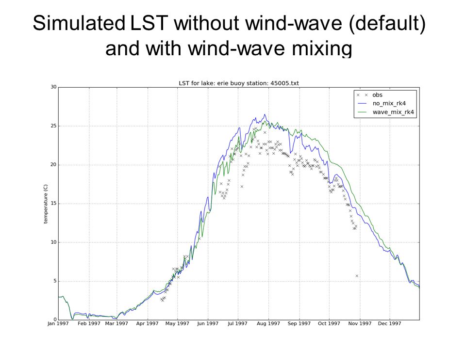
40. Simulated LST without wind-wave (default) and with wind-wave mixing

44. Simulated ice cover without wind-wave (default) and with wind-wave mixing

46. 7. Summary No a model is perfect, but can be improved and modified for a better numerical (schemes) and physical (dynamic processes) sound model An unstructured-grid FVCOM was implemented for all 5 lakes. The model-data comparison was conducted using EEGLE measurements in 1998, and from 1993-2008. FVCOM-ice was improved by changing the inertially-unstable Euler forward and runger-Kutta schemes  the most commonly-used 2 nd - order accuracy leapfrog scheme, and ice thermodynamics was also modified, because a neutral stable scheme is the best choice for all ocean processes Modified FVCOM-ice include surface wave mixing parameterization FVCOM-ice was run for 1993-1997, and the model-data comparison is being conducted

47. Future efforts Run the models to validate working scientific hypotheses using GLIM, ICEPOM, and FVCOM Run the models for climate studies from years to decades (1973- present) Couple FVCOM-ice to CWRF to conduct climate change studies and downscaling in the Great Lakes, and for future projection in 2040- 2070 using forcing derived from CWRF (Lofgren and Xiao) Provide seasonal projection of lake ice for both temporal and spatial distribution Couple (offline) FVCOM-ice with a well-tuned ecosystem model, Atlantis (Rutherford, Mason, Zhang) for GLRI Transfer to NOS for operational forecast (Anderson, Chu) and more …..

48. Question? Jia Wang, NOAA GLERL, 734-741-2281; jia.wang@noaa.gov Appreciate support from EPA-GLRI (Great Lakes Restoration Initiative) to climate study for decision making