1. Phase Space Representation of Quantum Dynamics Anatoli Polkovnikov, Boston University Seminar, U. of Fribourg 07/08/2010

2. Outline Quantum versus classical description of dynamics. Coherent states, duality of particle and wave classical limits. Phase space representation of quantum mechanics through the Wigner function. Von Neumann equation for the density matrix in the Wigner representation. Semiclassical (truncated Wigner) approximation. Path integral representation of the evolution. semiclassical approximation and beyond. Examples.

3. Two examples of complexity. Single neuron – relatively easy to characterize. ~10 10 neurons ??? NAND gate Computers are complicated, but we understand them Is “more” fundamentally different or just more complicated?

4. From single particle physics to many particle physics. Classical mechanics: Need to solve Newton’s equation (fully deterministic given initial conditions) Single particle Many particles Instead of one differential equation need to solve n differential equations, not a big deal!? The only uncertainty comes from potentially unknown initial conditions. Chaos impedes our ability to make long time accurate deterministic predictions.

5. Quantum mechanics: Need to solve Schrödinger equation. Exponentially large Hilbert space.M n Use specific numbers: M=200, n=100. Fermions: Bosons: QM gives fundamentally probabilistic description of evolution: we deal with combination of quantum-mechanical and probabilistic uncertainty.

6. Quantum systems: time evolution is trivial, complexity (chaos) is hidden in the many-body eigenstates and in exponentially large Hilbert space. Classical systems: states of the system are trivial (points in the phase space), time evolution is nontrivial. Dynamics

7. Expansion of quantum dynamics around classical limit. Classical (saddle point) limit: (i) Newtonian equations for particles, (ii) Gross-Pitaevskii equations for matter waves, (iii) Maxwell equations for classical e/m waves and charged particles, (iv) Bloch equations for classical rotators, etc. Questions: What shall we do with equations of motion? What shall we do with initial conditions? What shall we do with observables? Challenge : How to reconcile the exponential complexity of quantum many body systems and power law complexity of classical systems?

8. Coherent states. Dual classical corpuscular and wave limits. Bosonic creation-annihilation operators Classical limit: Basic representation: coherent states: Coordinate-momentum representation

9. Poisson Brackets and Equations of Motion Introduce As in the coordinate momentum representation in the classical limit

10. Equations of motion for operators Classical limit Recover Gross-Pitaevskii equation – classical wave equation for interacting bosons

11. Hamiltonian dynamics. Particle limitWave limit Phase space operators Canonical commutation relations Classical limit - Poisson brackets Classical limit – Equations of motion Newton’s equationsGP equations

12. (M. Greiner et. al., 2002 ). Superfluid-Insulator transition as an example of particle-wave duality. (M. Greiner et. al., 2002 ). Classical phase in terms of waves. Classical phase in terms of particles. Quantum phase transition

13. How can we connect classical and quantum description? Wigner function and Weyl ordering. G.S. of a harmonic oscillator: Wigner function can be interpreted as a quasi probability distribution.

14. Wigner function is the Weyl symbol of the density matrix Wigner function is analogous to the probability distribution. is not positive-definite – quasi-probability dsitribution. At finite T Wigner function becomes Bolzmann’s function – smooth connection of quantum and classical statistics. Facts about the Wigner function 1. 2. 3.

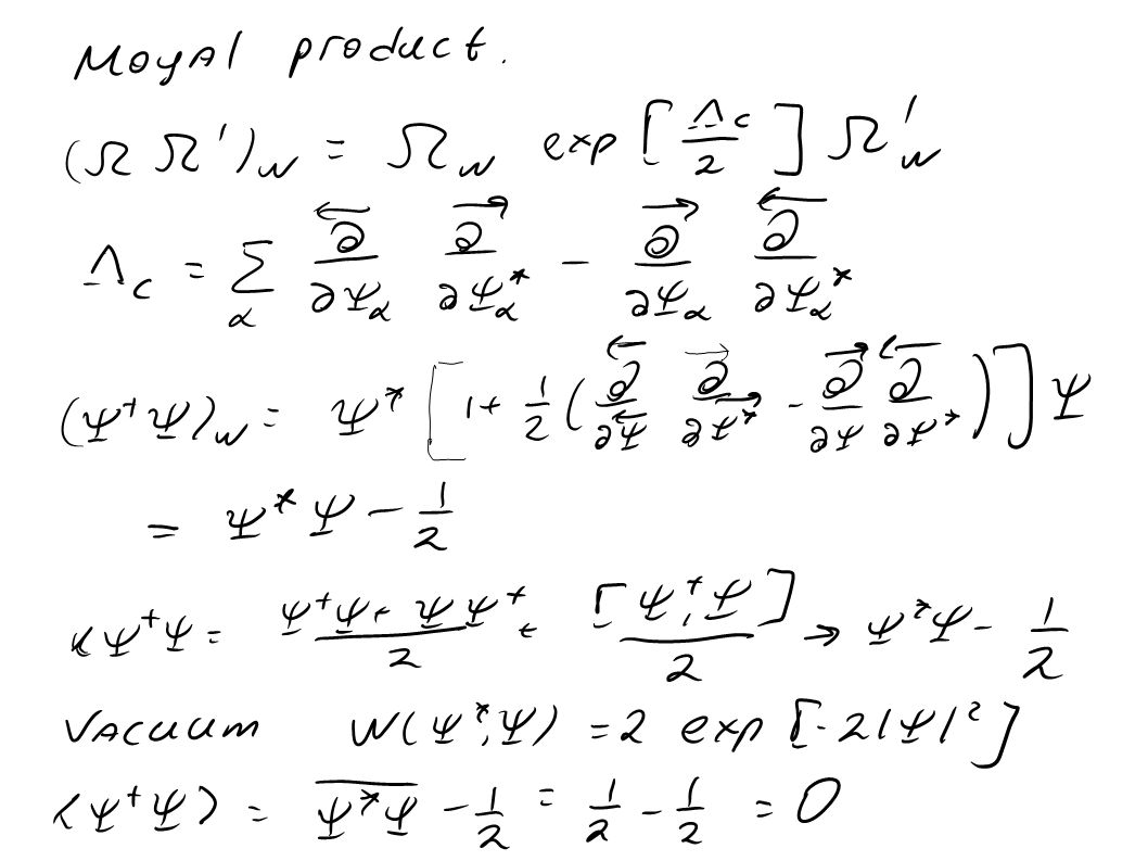
15. Expectation value of product of operators, Moyal product.   0 - Moyal product becomes ordinary product

16. Example

17. The Bopp representation of an operator reduces it to the classical function in the limit   0 and automatically reproduces the Weyl symbols of these operator.

18. Consider a coherent state as an example

19. Bopp operators for coherent states

20. Summary of phase space methods Wigner-Weyl quantization: Moyal product (basic multiplication rule) Bopp operators (basic representation)

21. Phase space methods and quantum dynamics Von Neumann equation for the density matrix Coherent states:

22. Expansion in  This equation can be solved using the method of characteristics, which are the classical trajectories.

23. Coherent states: Characteristics: W( ,  *,t)=const are given by the Gross-Pitaevskii equation Example

24. Semiclassical (truncated Wigner) approximation Quantum mechanics enters through 1.The Wigner function, which is different from the Boltzmann’s distribution, and which can be nonpositive. 2.Through the Weyl ordering of the Hamiltonian in the classical equations of motion. 3.Through the Weyl ordering of the observable Coherent states – same story:

25. Interpret this derivative as a response to the quantum jump

26. Combining left and right Bopp representations we find The last rule generalizes canonical commutation relations to non-equal times

28. Sketch of the path integral derivation of the time evolution. (Very similar to Keldysh formalism) Change variables

29. Wigner function and Weyl oredring emerg automatically from the boundary terms at  = 0 and  =t. No special assumptions are needed. For details of the derivation see: A.P. arXiv:0905.3384, Phys. Rev. A, vol. 68 (5), 053604 (2003).

30. Recover semiclassical approximation by expanding action to the linear order in quantum fields: Then functional integration is trivial: we are getting  -function constraints enforcing classical equations of motion:

31. Once again semiclassical – truncated Wigner – approximation The same story happens in the coherent state basis: integrating over the quantum field in the leading order enforces Gross- Pitaevskii equations on the classical fileds:

32. Non-equal time correlations functions (result) Recover Bopp operators (also automatically). Same for coherent states. Operator dependent jump at t=t 1

33. Beyond truncated Wigner approximation (TWA) Expand action to the third order in quantum fields (no corrections to TWA in harmonic theories)

34. Note that  plays the role of the correction to the conjugate momentum = quantum jump Higher order corrections – more jumps

35. Quantum corrections emerge as a nonlinear response to infinitesimal jumps in classical phase space variables. Each jump carries a factor of  2. Jumps do not affect short time behavior, i.e. TWA is asymptotically exact at short times. Equivalent representation through stochastic quantum jumps

36. Examples Classical equations of motion

38. More complicated example: sine-Gordon (Frenkel-Kontorova) model Assume initially V=0 and the system is in the ground state

39. Illustration: Sine-Grodon model, β plays the role of  V(t) = 0.1 tanh (0.2 t)

40. Turning on interactions in a system of interacting bosons Choose N=1 (per site), J=1, U 0 =1. Follow energy in the system.

41. Eight sites

42. 2D lattice 32x32 sites

43. Decoupling two 2D superfluids ( with L. Mathey )

44. Dicke model

45. Dicke model (many-level Landau-Zener problem) Consider (t)=-  t. Start in the with spin pointing up and no bosons. Classical limit: have exact solution b(t)=0, S z (t)=S, S x (t)=S y (t)=0. Quantum mechanically expect that at  0 – adiabatically follow the ground state:

46. The problem can be solved analytically using adiabatic invariants: A. Altland, V. Gurarie, T. Kriecherbauer, AP, PRA 79, 042703 (2009), A.P. Itin, P. Törmä, arXiv:0901.4778. Almost perfect agreement with the exact result in the whole range of 

47. TWA describes not only mean boson occupation but also fluctuations At slow rates distribution of bosons becomes Gumbel - extreme value statistics distribution.

48. Thermalization of bosons in an optical lattice. Prepare and release a system of bosons from a single site. Little evidence of thermalization in the classical limit. Strong evidence of thermalization in the quantum and semiclassical limits.

49. Many-site generalization 60 sites, populate each 10 th site.

50. Key points: 1) Hamiltonian dynamics. Particle limitWave limit Phase space operators Canonical commutation relations Classical limit - Poisson brackets Classical limit – Equations of motion Newton’s equationsGP equations

51. 2) Phase space representation of QM (naturally emerges from Feynman path interal) Wigner-Weyl quantization: Bopp operators: generate Weyl symbol. Provide natural interpretation of commutation relations through jumps in the classical phase space

52. Quantum corrections: nonlinear response or stochastic quantum jumps with non-positive probability. These methods are very useful to analyze various quantum (coherent) dynamical problems with initial conditions. Many applications to cold atoms. Open new possibilities. 3) Representation of quantum dynamics. Semiclassical approximation:

53. Example: Harmonic oscillator: