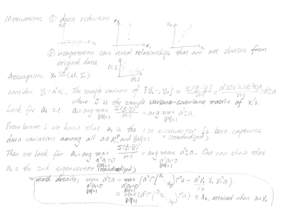
1. Stat240: Principal Component Analysis (PCA)

4. Open/closed book examination data >scores=as.matrix(read.table("http://www1.mat hs.leeds.ac.uk/~charles/mva- data/openclosedbook.dat", head=T)) >colnames(scores) >pairs(scores) MC VC LO NO SO 77 82 67 67 81 63 78 80 70 81 75 73 71 66 81 55 72 63 70 68 63 63 65 70 63 53 61 72 64 73 51 67 65 65 68......

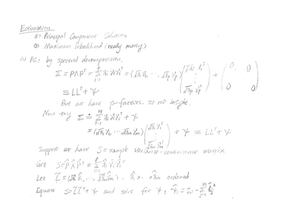
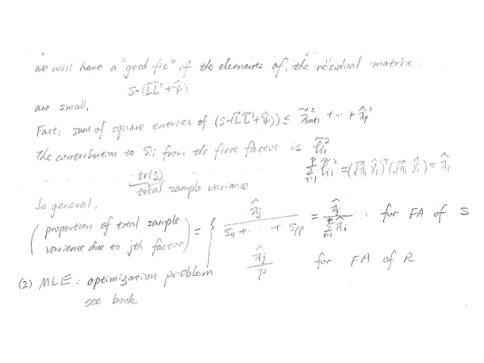
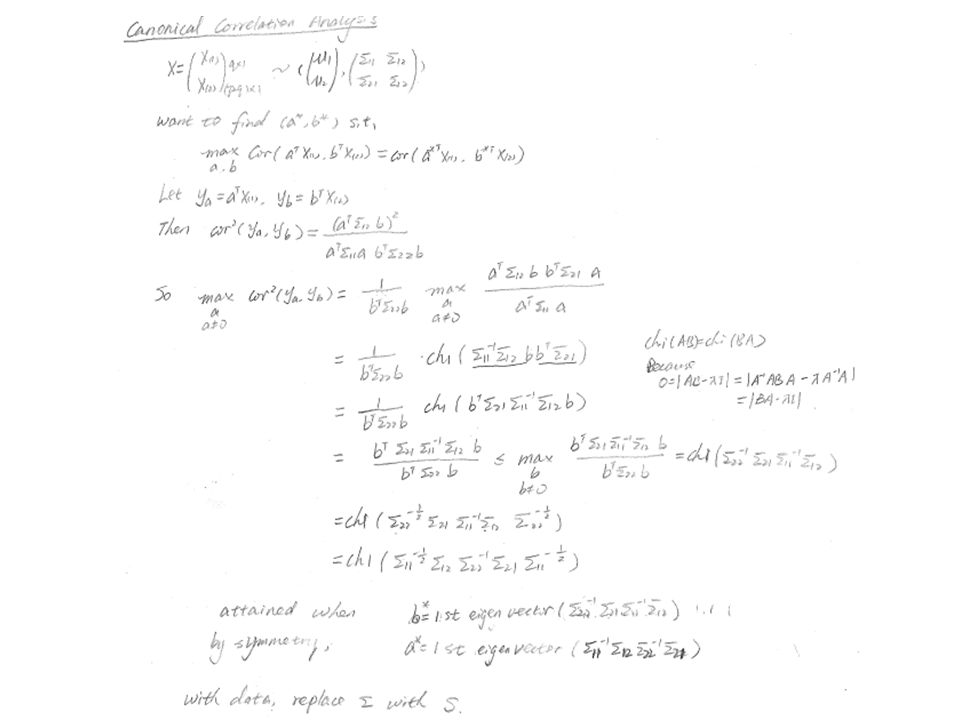
5. Sample Variance-Covariance > cov.scores=cov(scores) > round(cov.scores,2) MC VC LO NO SO MC 305.77 127.22 101.58 106.27 117.40 VC 127.22 172.84 85.16 94.67 99.01 LO 101.58 85.16 112.89 112.11 121.87 NO 106.27 94.67 112.11 220.38 155.54 SO 117.40 99.01 121.87 155.54 297.76 > eigen.value=eigen(cov.scores)$values > round(eigen.value,2) [1] 686.99 202.11 103.75 84.63 32.15 > eigen.vec=eigen(cov.scores)$vectors > round(eigen.vec,2) [,1] [,2] [,3] [,4] [,5] [1,] -0.51 0.75 -0.30 0.30 -0.08 [2,] -0.37 0.21 0.42 -0.78 -0.19 [3,] -0.35 -0.08 0.15 0.00 0.92 [4,] -0.45 -0.30 0.60 0.52 -0.29 [5,] -0.53 -0.55 -0.60 -0.18 -0.15 variances loadings

6. Principal Components PC1: PC2: PC3: PC4: PC5:

7. Scree plot >plot(1:5, eigen.value, xlab="i", ylab="variance", main="scree plot", type="b") > round(cumsum(eigen.value)/sum(eigen.value),3) [1] 0.619 0.801 0.895 0.971 1.000

8. “princomp” R has a function to conduct PCA > help(princomp) > obj=princomp(scores) > plot(obj, type= " lines " ) > biplot(obj)

9. PCA in checking MVN assumption By examining normality of PCs, especially the first two PCs. – Histograms, q-q plots – Bivariate plots – Checking outliers

10. PCA in regression Data: Y nx1, X nxp PCA is useful when we want to regress Y on a large number of independent variables (X) – Reduce dimension – Handle collinearity One would like to transform X to the principal components How to choose principal components?

11. PCA in regression A misconception: retain those with large variances – There is a tendency that PCs with large variances can better explain the dependent variable – But PCs with small variances might also have predictive value – Should consider largest correlation

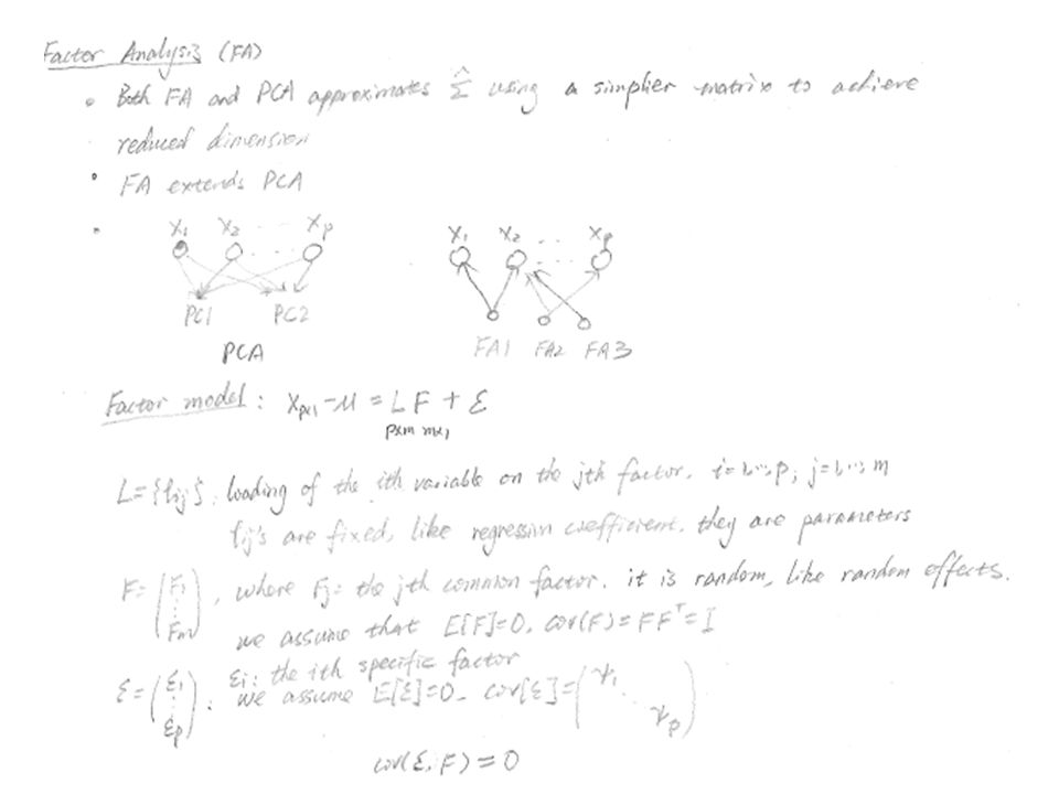
12. Factor Analysis (FA)

13. PCA vs FA Both attempt to do data reduction PCA leads to principal components FA leads to factors PCAFA X 1 X 2 X 3 X 4 PC 1 … … PC 4 X 1 X 2 X 3 X 4 F 1 F 2 F 3

18. FA in R The function is “factanal” Example: v1 <- c(1,1,1,1,1,1,1,1,1,1,3,3,3,3,3,4,5,6) v2 <- c(1,2,1,1,1,1,2,1,2,1,3,4,3,3,3,4,6,5) v3 <- c(3,3,3,3,3,1,1,1,1,1,1,1,1,1,1,5,4,6) v4 <- c(3,3,4,3,3,1,1,2,1,1,1,1,2,1,1,5,6,4) v5 <- c(1,1,1,1,1,3,3,3,3,3,1,1,1,1,1,6,4,5) v6 <- c(1,1,1,2,1,3,3,3,4,3,1,1,1,2,1,6,5,4) m1 <- cbind(v1,v2,v3,v4,v5,v6) obj=factanal(m1, factors=2) obj=factanal(covmat=cov(m1), factors=2) plot(obj$loadings,type="n“) text(obj$loadings,labels=c("v1", "v2", "v3", "v4", "v5","v6")) The default method is MLE The default rotation method used by “factanal” is varmax

19. Example: Examination Scores P=6: Gaelic, English, History, Arithmetic, Algebra, Geometry N=220 male students R= 1.0.439.410.288.329.248.4391.0.351.354.320.329.410.3511.0.164.190.181.288.354.1641.0.595.470.329.320.190.5951.0.464.248.329.181.470.4641.0

20. Factor Rotation Motivation: get better insights Varimax criterion – The rotation that maximizes the total variance of squares of (scaled) loadings