1. Chapter 2 Simulation Examples

2. Simulation steps using Simulation Table 1.Determine the characteristics of each of the inputs to the simulation (probability distributions). 2.Construct a simulation table (repetition 1). 3.For each repetition i, generate a value for the inputs, and evaluate function, calculating a value of response yi.

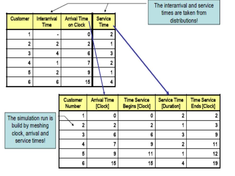
3. Simulation Table

4. Simulation of Queuing System (Details in chapter 6) Simple single server queuing system

5. Single server queue Calling population is infinite-Arrival rate does not change Units are served according FIFO Arrivals are defined by the distribution of the time between arrivals - inter-arrival time Service times are according to distribution Arrival rate must be less than service rate- stable system

6. Queueing system state –System Server Units (in queue or being served) Clock –State of the system Number of units in the system Status of server (idle, busy) –Events Arrival of a unit Departure of a unit

7. Arrival Event If server idle customer gets service, otherwise customer enters queue. Unit actions upon arrival

8. Departure Event If queue is not empty begin servicing next unit, otherwise server will be idle. Server Outcomes after departure

9. Grocery Store Example(Ex 2.1)

10. Producing Random Numbers from Random Digits Select randomly a number, e.g. 99219 - One digit: 0.9 - Two digits: 0.19 -Three digits: 0.219 Proceed in a systematic direction, e.g. - first down then right - first up then left

13. Example1: A Grocery Store

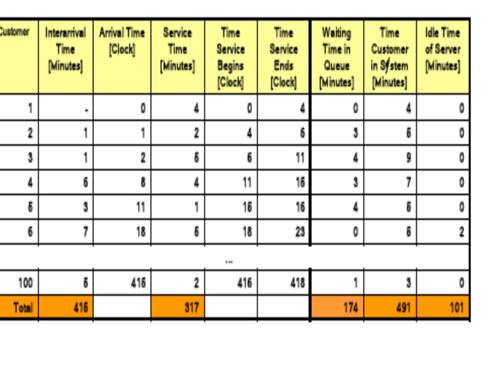
15. Average waiting time Probability that a customer has to wait Proportion of server idle time Average service time

16. Average time between arrivals Average waiting time of those who wait Average time a customer spends in system

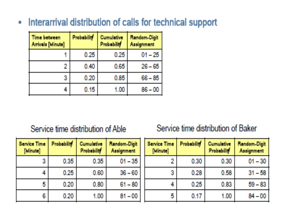
17. Example 2: Call Center Problem Consider a Call Center where technical personnel take calls and provide service Two technical support people (2 server) exists – Able – more experienced, provides service faster – Baker – newbie, provides service slower Rule – Able gets call if both people are idle Find out how well the current arrangement works

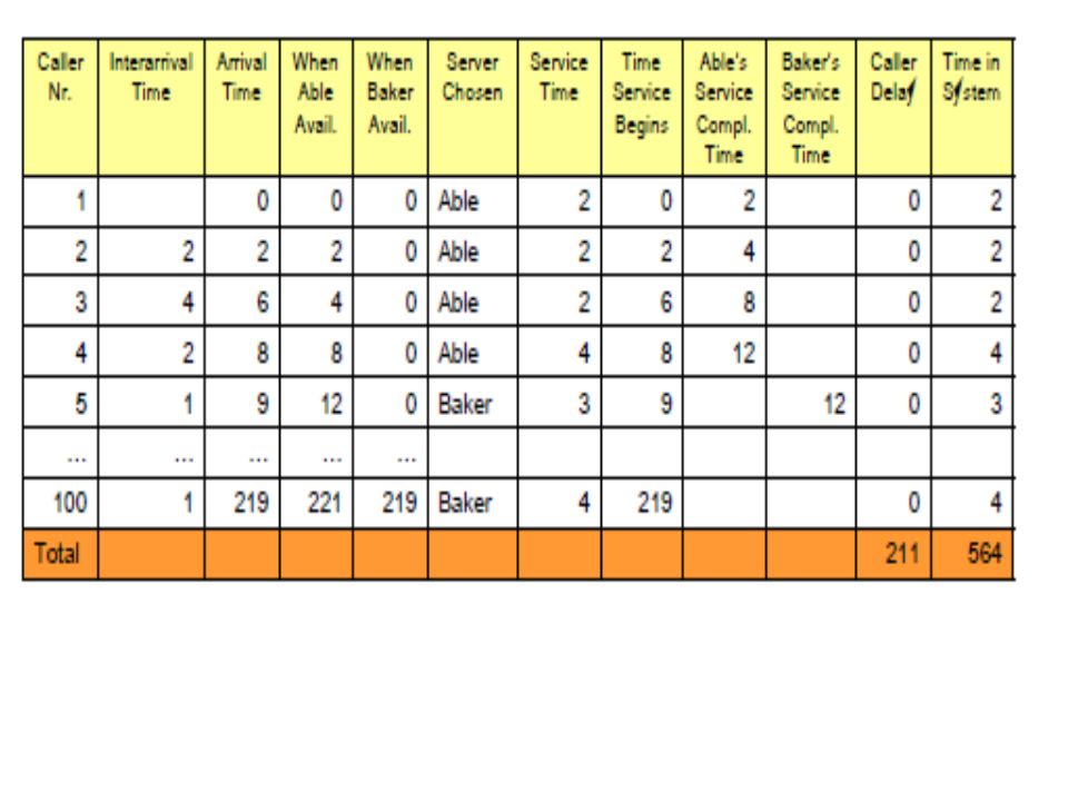
19. Simulation proceeds as follows Step 1: –For Caller k, generate an interarrival time Ak. Add it to the previous arrival time Tk-1 to get arrival time of Caller k as Tk = Tk-1 + Ak Step 2: – If Able is idle, Caller k begins service with Able at the current time Tnow – Able‘s service completion time Tfin,A is given by Tfin,A= Tnow+ Tsvc,A where Tsvc,A is the service time generated from Able‘s service time distribution. Caller k’s waiting time is Twait = 0. – Caller k‘s time in system, Tsys, is given by Tsys = Tfin,A – Tk – If Able is busy and Baker is idle, Caller begins with Baker. The remainder is in analogous. Step 3: – If Able and Baker are both busy, then calculate the time at which the first one becomes available, as follows: Tbeg = min(Tfin,A, Tfin,B) – Caller k begins service at Tbeg. When service for Caller k begins, set Tnow = Tbeg. – Compute Tfin,A or Tfin,B as in Step 2. – Caller k’s time in system is Tsys = Tfin,A – Tk or Tsys = Tfin,B - Tk

21. Example 3: Inventory System Important class of simulation problems: inventory systems A simple inventory system with  Lead time=0  order quantities are probabilistic  Demand is uniform over the time period Parameters – N Review period length – M Standard inventory level – Qi Quantity of order i

22. To avoid shortages, a buffer stock is needed Cost of stock  Interest on funds  Storage space  Guards Alternative: To make more frequent reviews  Ordering cost  Cost in being short Performance measure: Total cost (or total profit) Events in an (M, N) inventory system are – Demand for items – Review of the inventory position – Receipt of an order at the end of each review

23. Example 2.3 Newspaper sellers Problem