Download presentation
Presentation is loading. Please wait.

1
TIRGUL 10 Dijkstra’s algorithm Bellman-Ford Algorithm 1

2
Weighted distance Until now we have only considered unweighted graphs. Today we will focus on weighted graphs. Reminder: a weighted graph is G=(V,E,W), where W:VxV ℝ. For now, we will assume that for all w ∈ W, w>0 That is, every edge gets a positive number representing it’s weight.
, where W:VxV ℝ. For now, we will assume that for all w ∈ W, w>0 That is, every edge gets a positive number representing it’s weight..")
3
Weighted paths Definition: the weight of a path v 1 v 2 … v k is equal to the sum of weights: W(v 1 v 2 )+W(v 2 v 3 )+…+W(v k-1 v k ) Definition: the weighted distance between two nodes in a graph is the minimal weight of all paths between them. This is a natural extension of the notion of distance in unweighted graphs. Today we will see how to compute the weighted distance of all nodes from a given node s in a weighted graph G. Notations: (v) – v’s real weighted distance from s [v] – the algorithm’s answer regarding v’s distance from s.
 – v’s real weighted distance from s [v] – the algorithm’s answer regarding v’s distance from s..")
4
Finding the minimal weighted distance In unweighted graphs we used BFS to compute the distance between a node v and all other nodes. Q: Can we use it on weighted graphs by adding up weights as we go? A: no! Example: s a b 4 2 1 =4 = 2 =3

5
Insights Why does this fail? Visiting a first fails since we marked it as ‘visited’. Insight #1: a given distance cannot be fixed - we need to be able update it’s distance once we find shorter path s a b 4 2 1 4 2 3

6
Insights Let’s expand our example and run BFS with updates: The a c update did not help since a’s distance was wrong at the time of update. Notice that if we first expand b and then a, it does work. s a b c 4 2 1 1 5 4 2 5 3 4

7
Insights Let’s expand our example and run BFS with updates: The a c update did not help since a’s distance was wrong at the time of update. Notice that if we first expand b and then a, it does work. s a b c 4 2 1 1 5 4 2 5 3 4

8
Insights Insight #2: allowing distance updates is not enough – we must visit nodes in a certain order. Q: Is it true that there always exists an ordering such that BFS returns the correct weighted distances? A: YES! s a b c 4 2 1 1 5 4 2 5 3 4

9
Insights But what is a good order? We saw that updates can be ‘missed’ – when does this happen? Insight #3: if we went through the nodes in order of their actual distance, we would never miss an update. But finding the distance is the problem itself… s a b c 4 2 1 1 5 4 2 5 3 4

10
Locality and greediness Global order looks hard to find – what about local order? Insight #4: After expanding s: b is the node with the smallest current [ ] value b‘s [ ] value is equal to it’s real distance b is also the next yet to be expanded node in the ordering by If we choose b next, we won’t miss any updates! Is this always true? s a b c 4 2 1 1 4 4 2

11
Proposed ‘greedy’ solution At every step we will have: A - Nodes we’ve expanded B - Nodes we’ve visited C - Nodes we haven’t visited yet At each step we will: Expand the node v ∈ B with the current smallest [ ] Update the [ ] value of it’s neighbors from B Visit it’s neighbors from C and update their [ ] values Move v to A We’ll need to show that when a node is added to A, d=. Greedy!
![Proposed ‘greedy’ solution At every step we will have: A - Nodes we’ve expanded B - Nodes we’ve visited C - Nodes we haven’t visited yet At each step we will: Expand the node v ∈ B with the current smallest [ ] Update the [ ] value of it’s neighbors from B Visit it’s neighbors from C and update their [ ] values Move v to A We’ll need to show that when a node is added to A, d=.](http://images.slideplayer.com/36/10631211/slides/slide_11.jpg "Greedy!.")
12
Algorithm: AlmostDijkstra(G,s) For all v ≠ s [v]= ∞ [s] = 0 A =, B = {s}, C = V\S While B ≠ Choose v ∈ B with minimal [ ] For all neighbors u ∈ B,C of v [u] = min([u], [v]+W(v,u)) if u ∈ C, move u into B Move v from B to A
![Algorithm: AlmostDijkstra(G,s) For all v ≠ s [v]= ∞ [s] = 0 A =, B = {s}, C = V\S While B ≠ Choose v ∈ B with minimal [ ] For all neighbors u ∈ B,C of v [u] = min([u], [v]+W(v,u)) if u ∈ C, move u into B Move v from B to A](http://images.slideplayer.com/36/10631211/slides/slide_12.jpg "Algorithm: AlmostDijkstra(G,s) For all v ≠ s [v]= ∞ [s] = 0 A =, B = {s}, C = V\S While B ≠ Choose v ∈ B with minimal [ ] For all neighbors u ∈ B,C of v [u] = min([u], [v]+W(v,u)) if u ∈ C, move u into B Move v from B to A")
13
Proof of correctness Lemma 1: a sub-path of a shortest path is also a shortest path Proof: take p=x … y … z, p’=x … y. by contradiction there exists a path q from x to y with len(q)<len(p’), then the path q with y … z is shorter than p. This contradicts p being a shortest path. Lemma 2: for all v ∈ V, in every step, (v)<=d(v) Proof: at the begging, [s]=0=(s), and for all v ≠ s, [v] = ∞ ≥ (v). Since values are changed by updates, assume by contradiction v is the first node updated such that [v]<(v). Since v was updated (assume by u): [u]+w(u,v) = [v] < (v) ≤ (u)+w(u,v) ⇒ [u] < (u) in contradiction to v being the first with <.
<len(p’), then the path q with y … z is shorter than p. This contradicts p being a shortest path. Lemma 2: for all v ∈ V, in every step, (v)<=d(v) Proof: at the begging, [s]=0=(s), and for all v ≠ s, [v] = ∞ ≥ (v). Since values are changed by updates, assume by contradiction v is the first node updated such that [v]<(v). Since v was updated (assume by u): [u]+w(u,v) = [v] < (v) ≤ (u)+w(u,v) ⇒ [u] < (u) in contradiction to v being the first with <..")
14
Proof of correctness Induction on n=|A|. Claim: All nodes in A have a correct [ ] value Basis: n=1, A={s}, and [s] = 0 = (s). Step: we will assume for all k<n, and prove for n. Let v be the n’th node inserted into A. Let p be a true shortest weighted path between s and v. Case 1 - p ⊆ A: Before inserting v into A it’s size was less than n, so by the induction assumption for all w ∈ A, [w] = (w). Let u be the node before v in p. Since u ∈ A, by the above [u] = (u). Since v is a neighbor of u, when u was inserted into A, v’s [ ] value was updated. Since (u,v) ∈ p and p is a shortest path, after the update [v] ≤ (v). From lemma 1 [v] ≥ (v), therefore [v] = (v).
. Step: we will assume for all k<n, and prove for n. Let v be the n’th node inserted into A. Let p be a true shortest weighted path between s and v. Case 1 - p ⊆ A: Before inserting v into A it’s size was less than n, so by the induction assumption for all w ∈ A, [w] = (w). Let u be the node before v in p. Since u ∈ A, by the above [u] = (u). Since v is a neighbor of u, when u was inserted into A, v’s [ ] value was updated. Since (u,v) ∈ p and p is a shortest path, after the update [v] ≤ (v). From lemma 1 [v] ≥ (v), therefore [v] = (v)..")
15
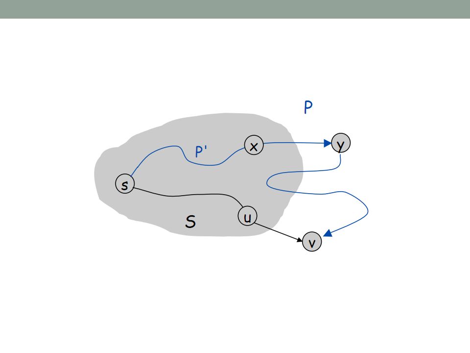
Proof of correctness Case 2 - p ⊈ A: By contradiction, assume v is inserted into A with a wrong [ ]. Let y be the first node in p that is not in A (y ≠ v, otherwise we’d be in case 1). s ∈ A, so A is not empty. Therefore, let x be y’s predecessor in p, so (x,y) ∈ E, x ∈ A. Since x ∈ A, and since x was inserted into A when it’s size was less than n, by the induction assumption it’s [x] = (x). Consider (y) and [y]. From lemma 2, (y) ≤ [y]. From lemma 1, the sub-path p’=s … x y ⊈ p is a shortest path from s to x. Since all of x’s neighbors (including y) were updated when x was inserted into A, and at that time [x]=(x), after the update [y]=(y) (From lemma 1 again, any other update could not have resulted in [y]<(y) ).
![Proof of correctness Case 2 - p ⊈ A: By contradiction, assume v is inserted into A with a wrong [ ].](http://images.slideplayer.com/36/10631211/slides/slide_15.jpg "Let y be the first node in p that is not in A (y ≠ v, otherwise we’d be in case 1). s ∈ A, so A is not empty. Therefore, let x be y’s predecessor in p, so (x,y) ∈ E, x ∈ A. Since x ∈ A, and since x was inserted into A when it’s size was less than n, by the induction assumption it’s [x] = (x). Consider (y) and [y]. From lemma 2, (y) ≤ [y]. From lemma 1, the sub-path p’=s … x y ⊈ p is a shortest path from s to x. Since all of x’s neighbors (including y) were updated when x was inserted into A, and at that time [x]=(x), after the update [y]=(y) (From lemma 1 again, any other update could not have resulted in [y]<(y) )..")
16
Proof of correctness Since the length of p’ is less than p, since they are both shortest paths, and since w>0, we get that (y) < (v). Since from lemma 1 (v) ≤ [v], we get that: [y] = (y) < (v) ≤ [v] So [y]< [v],in contradiction to the algorithm choosing the node with the smallest [ ] value. Therefore, (v) = [v].
 ≤ [v], we get that: [y] = (y) < (v) ≤ [v] So [y]< [v],in contradiction to the algorithm choosing the node with the smallest [ ] value. Therefore, (v) = [v]..")
18
Choosing wisely In each step we need to choose v in B with the minimal [ ] value. Nodes are moved from C to B [ ] values of nodes are updated all the time. Q: What data structure gives these functions at a good running time? A: Priority queue! Using a binary min-heap we get: ExtractMin – O(logn) Insert – O(logn) DecreaseKey – O(logn) Notice that our algorithm is actually BFS with a priority queue (instead of a regular queue).
![Choosing wisely In each step we need to choose v in B with the minimal [ ] value.](http://images.slideplayer.com/36/10631211/slides/slide_18.jpg "Nodes are moved from C to B [ ] values of nodes are updated all the time. Q: What data structure gives these functions at a good running time. A: Priority queue. Using a binary min-heap we get: ExtractMin – O(logn) Insert – O(logn) DecreaseKey – O(logn) Notice that our algorithm is actually BFS with a priority queue (instead of a regular queue)..")
19
19 Dijkstra’s Algorithm Input: graph G=(V,E,W), directed or undirected Starting node s W consists of positive edges Output: for each node v ∈ V: It’s weighted distance from s A shortest weighted path from s
, directed or undirected Starting node s W consists of positive edges Output: for each node v ∈ V: It’s weighted distance from s A shortest weighted path from s")
20
Dijkstra(G,s) for all u V : [u] = ∞ [s] = 0 H = buildPriorityQueue(V) // using [ ]-values as keys while H ≠ : u = extractMin(H) for all edges (u,v) E: if [v] > [u] + w(u,v): [v] = [u] + w(u,v) decreaseKey(H, v, [v]) 20
![Dijkstra(G,s) for all u V : [u] = ∞ [s] = 0 H = buildPriorityQueue(V) // using [ ]-values as keys while H ≠ : u = extractMin(H) for all edges (u,v) E: if [v] > [u] + w(u,v): [v] = [u] + w(u,v) decreaseKey(H, v, [v]) 20](http://images.slideplayer.com/36/10631211/slides/slide_20.jpg "Dijkstra(G,s) for all u V : [u] = ∞ [s] = 0 H = buildPriorityQueue(V) // using [ ]-values as keys while H ≠ : u = extractMin(H) for all edges (u,v) E: if [v] > [u] + w(u,v): [v] = [u] + w(u,v) decreaseKey(H, v, [v]) 20")
21
Dijkstra-Running Example 21 C 8 1 5 A 2 4 BD E 3 A:0 B:∞ C:∞ D:∞ E: ∞ A:0 B:4 C:2 D:8 E: 7 A:0 B:4 C:2 D:10 E: 7 A:0 B:4 C:2 D:∞ E: ∞

22
Dijkstra-Complexity Dijkstra's algorithm is structurally identical to BFS. However, it is slower because the priority queue is computationally more demanding than the constant-time pop and push of BFS. Runtime analysis using a binary heap: BuildPriorityQueue takes O(|V|). ExtractMin and Insert are executed |V| times each – once for each node, thus it takes O(|V|log|V|). In the worst case, DecreaseKey can be executed for every edge, thus |E| times, giving O(|E|log|V|). Overall we get O((|V|+|E|)log|V|) 22
. ExtractMin and Insert are executed |V| times each – once for each node, thus it takes O(|V|log|V|). In the worst case, DecreaseKey can be executed for every edge, thus |E| times, giving O(|E|log|V|). Overall we get O((|V|+|E|)log|V|) 22.")
23
Negative Weights Q: Can Dijkstra work with negative weights? A: No! for example: 23 s 7 2 -2 5 6 6 7 5 And this is wrong! 7 3 4

24
Bellman-Ford Algorithm Input: Directed graph G = (V,E) edge lengths {w e :e E} with no negative cycles vertex s V Output: For all vertices u reachable from s, [u] is set to the distance from s to u. 24
![Bellman-Ford Algorithm Input: Directed graph G = (V,E) edge lengths {w e :e E} with no negative cycles vertex s V Output: For all vertices u reachable from s, [u] is set to the distance from s to u.](http://images.slideplayer.com/36/10631211/slides/slide_24.jpg "24.")
25
Bellman-Ford Algorithm Idea At a given time we have a “guess” of the shortest paths from s to other vertices. We go over edges and see if they can improve our guess This must be repeated many times 25 2 1 1 3 3 1 12 6 7 s v w x b c d a 3 3 6 1 1 2 6 2 54

26
Bellman-Ford(G,w,s) for all u V : [u] = ∞ [s] = 0 repeat |V|-1 times for all (u,v) E: [v] = min{[v], [u] + w(u,v)} 26
![Bellman-Ford(G,w,s) for all u V : [u] = ∞ [s] = 0 repeat |V|-1 times for all (u,v) E: [v] = min{[v], [u] + w(u,v)} 26](http://images.slideplayer.com/36/10631211/slides/slide_26.jpg "Bellman-Ford(G,w,s) for all u V : [u] = ∞ [s] = 0 repeat |V|-1 times for all (u,v) E: [v] = min{[v], [u] + w(u,v)} 26")
27
Running Example sbacde 0 0263 021344 021123 27 s b c e d 3 6 2 6 -2 2 2 2 1 a

28
Bellman Ford & Negative cycles When there is a negative cycle in a graph shortest path are not (well) defined. How can the algorithm detect negative cycles ? Such a cycle would allow us to endlessly apply rounds of update operations, reducing [ ] estimates every time. So instead of stopping after |V|-1 iterations, perform one extra round. There is a negative cycle if and only if some [ ] value is reduced during this final round. 28 s 2 2 3 6 2 -5

29
Bellman Ford-Complexity for all u V : [u] = ∞ [s] = 0 repeat |V|-1 times for all (u,v) E: [v] = min{[v], [u] + w(u,v)} 29 O)|E||V|)
![Bellman Ford-Complexity for all u V : [u] = ∞ [s] = 0 repeat |V|-1 times for all (u,v) E: [v] = min{[v], [u] + w(u,v)} 29 O)|E||V|)](http://images.slideplayer.com/36/10631211/slides/slide_29.jpg "Bellman Ford-Complexity for all u V : [u] = ∞ [s] = 0 repeat |V|-1 times for all (u,v) E: [v] = min{[v], [u] + w(u,v)} 29 O)|E||V|)")
Similar presentations


 : weighted, directed graph w : E R : weight function P=>")


 Problem Application of s-s-s-p for Solving a System of Difference Constraints.>")


 Spanning tree of graph G is tree T = (V,E T E, R) –Tree has same set.>")
 sample questions. DAST 2005 Q.We’ve seen that solving the shortest paths problem requires O(VE) time using the Belman-Ford.>")