1. Energy inputs from Magnetosphere to the Ionosphere/Thermosphere ASP research review Yue Deng April 12 nd, 2007

2. 1.Introduction: Earth-Sun System Earth and Sun not to scale Solar Wind Magnetosphere Ionsophere/ Thermosphere

3. Solar Wind - Solar wind is always coming out of the sun in a spiral motion (ballerina skirt) - Plasma (H + (p + ) and e - ) - An interplanetary magnetic field (IMF) is brought with the plasma

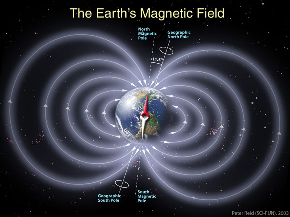
5. The solar wind and IMF interact with Earth’s magnetic field It is Earth’s magnetic field (Magnetosphere) that protects us and our satellites from the solar wind, CMEs and solar flares.

6. If the IMF is oriented correctly (southward) there is magnetic reconnection on the dayside. The solar wind electrons then travel down these connected (open) field lines and interact with the ionosphere. This causes the aurora. The color of the aurora is determined by the molecule the electron excites.

7. The aurora is a beautiful light show for one and all.

8. Thermosphere-Ionosphere Overview Thermosphere-Ionosphere Overview Courtesy of Stan Solomon, HAO

9. Earth’s Ionosphere/Thermosphere Processes Courtesy of Joseph Grebowsky, NASA GSFC Electrodynamics & particle Sun Tides and Gravity Waves

11. Reasons for underestimating of Joule heating in global models Reasons for underestimating of Joule heating in global models E-field temporal variability Spatial resolution Vertical velocity difference

12. Underestimation of Joule heating Main method of energy transport: for Jan. 1997 storm Joule heating is 47% (Lu et al., [1998]). Main method of energy transport: for Jan. 1997 storm Joule heating is 47% (Lu et al., [1998]). Primary driver of global thermosphere- ionosphere disturbance. (Banks, [1977]) Primary driver of global thermosphere- ionosphere disturbance. (Banks, [1977])

13. The Global Ionosphere-Thermosphere Model (GITM) GITM solves for: 6 Neutral & 5 Ion Species 6 Neutral & 5 Ion Species Neutral winds Neutral winds Ion and Electron Velocities Ion and Electron Velocities Neutral, Ion and Electron Temperatures Neutral, Ion and Electron Temperatures GITM Features: Flexible grid resolution Flexible grid resolution Solves in Altitude coordinates Solves in Altitude coordinates Can have non-hydrostatic solution Can have non-hydrostatic solution Coriolis Coriolis Vertical Ion Drag Vertical Ion Drag Non-constant Gravity Non-constant Gravity Massive heating in auroral zone Massive heating in auroral zone Runs in 1D and 3D Runs in 1D and 3D Vertical winds for each major species with friction coefficients Vertical winds for each major species with friction coefficients Non-steady state explicit chemistry Non-steady state explicit chemistry Variety of high-latitude and Solar EUV drivers Variety of high-latitude and Solar EUV drivers Fly satellites through model Fly satellites through model

14. Case 1: ConstCase 2: SinCase 3: Multi Vsw=400km/s, IMF(By)=0nT, F10.7=150, HPI=10GW IMF(B z )= -0.5  -6.5 nT A 0 = -6.5nT IMF(B z )=A 0 +A 1 Cos(2πt/T 1 ) A 0 = -6.5nT A 1 = 4.0nT, T 1 = 4.0 Hour IMF(B z )=A 0 +A 1 Cos(2πt/T 1 ) +A 2 Cos(2πt/T 2 ) A 0 = -6.5nT A 1 = 4.0nT, T 1 = 4.0 Hour A 2 = 2.0nT, T 2 = 40 Min (1) Effect of E-field temporal variability

15. Comparison: Fd Fd [Codrescu,95] 8 Hour period averages of E are the same 8 Hour period averages of E are the same Sigma(E)/ave r(E) is 32%,36% Sigma(E)/ave r(E) is 32%,36% Joule heating increases: 17%, 22%. Joule heating increases: 17%, 22%. Joule heating rates are different from Joule heating rates are different from Case 1 Case 2 Case 3

16. (2) Spatial Resolution (Lon * Lat) 5 0 * 1.25 0 5 0 * 2.5 0 5 0 * 5 0  Maximum increases from 0.11  0.14  0.15 W/kg  At 200km, resolution can cause 22% difference.

17. (3) Magnetic Dip Angle 3-D 2-D Difference  3-D and 2-D results are similar, difference is not big  Altitude profile shows some difference to Joule heating  Increased percentage is close to 3%.

18. Conclusions Temporal Variability of E-field definitely increases the Joule heating. Temporal Variability of E-field definitely increases the Joule heating. Spatial resolution of GCM can make some difference to the calculated Joule heating. Spatial resolution of GCM can make some difference to the calculated Joule heating. Vertical component velocity has very small effect. Vertical component velocity has very small effect.

19. Joule heating VS. Poynting flux Joule heating VS. Poynting flux

20. J. Thayer, JGR 2000.

21. New empirical electrodynamic model (DE-2). The distributions of altitude-integrated Joule heating and Poynting flux are different. The total energy from Poynting flux is 40% larger than the energy of Joule heating.

22. Coupled with NCAR_TIEGCM. The difference depends on the altitude and season. The difference depends on the altitude and season. The hemispheric average of the temperature increases by around 50 K. The hemispheric average of the temperature increases by around 50 K.

23. 2-D Poynting flux  3-D energy input 2-D Poynting flux  3-D energy input Impact depends on the distributing method. Impact depends on the distributing method.

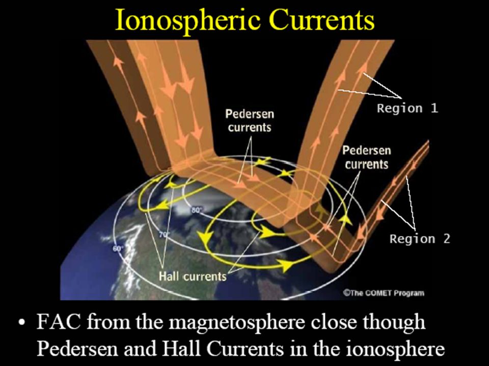
24. What Coupling Should Be Magnetosphere Model Field-aligned Currents Heat Flux Electron & Ion Precipitation Plasmasphere Density Potential Electrodynamics Model Ionosphere-Thermosphere Model Neutral wind FACs Conductances Upward Ion Fluxes TidesGravity Waves Solar Inputs PhotoelectronFlux Courtesy of Aaron Ridley, University of Michigan

25. Thank you!

26. Three-dimensional schematic view of the magnetosphere.