Download presentation
Presentation is loading. Please wait.

1
Mitesh Patel Co-Authors: Steve Warren, Daniel Mortlock, Bram Venemans, Richard McMahon, Paul Hewett, Chris Simpson, Rob Sharpe m.patel06@imperial.ac.uk

3
Neutral hydrogen clumps absorb hydrogen at the clump redshift Produces absorption blueward of the emission redshift

4
Neutral hydrogen clumps absorb hydrogen at the clump redshift Produces absorption blueward of the emission redshift Many clumps leads to complete absorption blueward of Ly Ly forest Venemans et al. (2007)
.")
5
Fan et al. (2006)
")
6
Optical surveys are limited to z- band dropouts UKIRT Infra-red Deep Sky Survey Wide field Imager At least 3 magnitudes deeper than 2MASS in J,H and K Consists of 5 mini-surveys Galactic Clusters Survey (GCS) Galactic Plane Survey (GPS) Deep Extragalactic Survey (DXS) Ultra Deep Survey (UDS) Large Area Survey (LAS) www.ukidss.org
 Galactic Plane Survey (GPS) Deep Extragalactic Survey (DXS) Ultra Deep Survey (UDS) Large Area Survey (LAS)")
7
http://surveys.roe.ac.uk/wsa/index.html

8
Observes Y (20.2), J (19.6), H (18.8) and K (18.2) Aims to cover 4000 deg 2 Area also covered by SDSS DR5: observed 1270 deg 2 in all four bands
, J (19.6), H (18.8) and K (18.2) Aims to cover 4000 deg 2 Area also covered by SDSS DR5: observed 1270 deg 2 in all four bands")
9
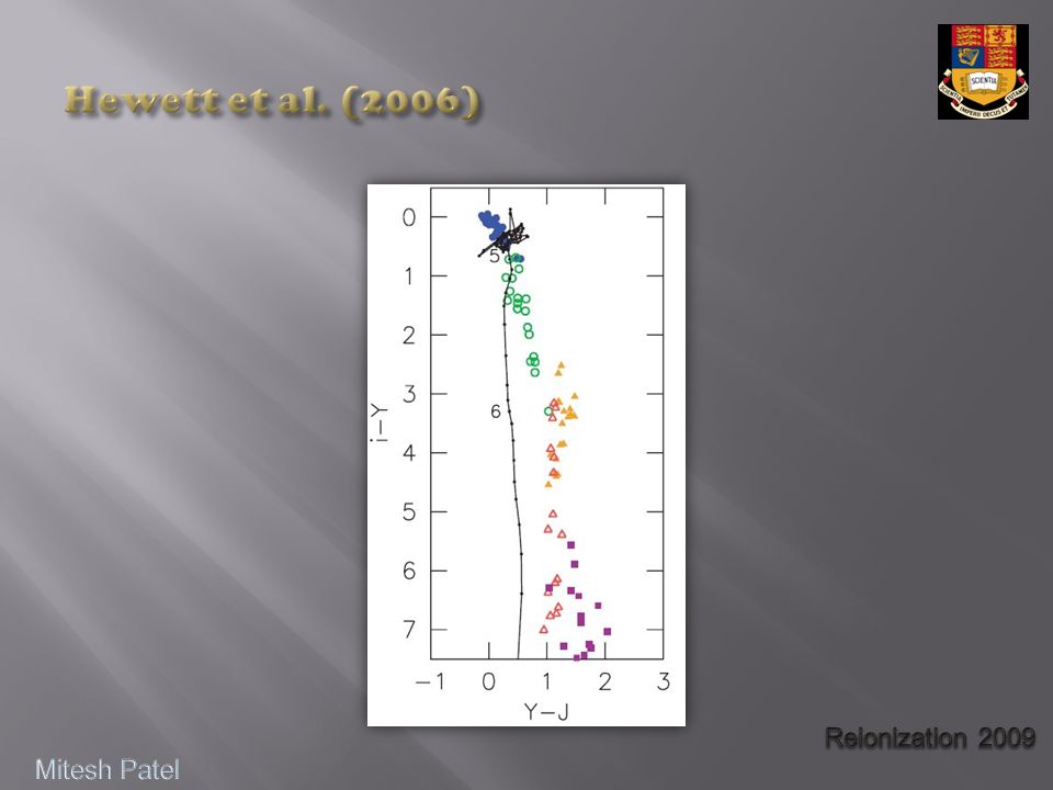
Use models by Hewett & Madison (2005) and look at expected colours Use both SDSS and UKIDSS tables Find objects with red i-Y colours and blue Y-J colours Hewett et al. (2006)
.")
10
Use models by Hewett & Madison (2005) and look at expected colours Use both SDSS and UKIDSS tables Find objects with red i-Y colours and blue Y-J colours Hewett et al. (2006)
.")
13
Mortlock et al. (2009) z = 6.127
 z = 6.127")
14
F 0.32

15
Mg II (2798 A) Central Wavelength = 19940 +/- 12 A EW = 14 A Redshift = 6.127 +/- 0.004
 Central Wavelength = /- 12 A EW = 14 A Redshift = /")
16
DR 5 candidate Re-observed in Y + J Confirmed quasar-like colors

17
DR 5 candidate Re-observed in Y + J Confirmed quasar-like colors Redshift = 6.04 from Ly Warren et al. (in prep)
.")
18
SDSS found a number of quasars Follow the analysis of Fan et al. (2006) Fit a power law to the quasar continuum Select an upper limit redshift not affected by Ly Take a region size of z = 0.15 Measure the ratio of the original flux to the absorbed flux Take multiple regions, up to a lower limit at Ly
 Fit a power law to the quasar continuum Select an upper limit redshift not affected by Ly Take a region size of z = 0.15 Measure the ratio of the original flux to the absorbed flux Take multiple regions, up to a lower limit at Ly .")
19
Fan et al. (2006) Fit a power law to the quasar continuum Select an upper limit redshift not affected by Ly Take a region size of z = 0.15 Measure the ratio of the original flux to the absorbed flux Take multiple regions, up to a lower limit at Ly
 Fit a power law to the quasar continuum Select an upper limit redshift not affected by Ly Take a region size of z = 0.15 Measure the ratio of the original flux to the absorbed flux Take multiple regions, up to a lower limit at Ly .")
20
Fan et al. (2006) Fit a power law to the quasar continuum Select an upper limit redshift not affected by Ly Take a region size of z = 0.15 Measure the ratio of the original flux to the absorbed flux Take multiple regions, up to a lower limit at Ly
 Fit a power law to the quasar continuum Select an upper limit redshift not affected by Ly Take a region size of z = 0.15 Measure the ratio of the original flux to the absorbed flux Take multiple regions, up to a lower limit at Ly .")
21
-ln (tfr) Fan et al. (2006)
 Fan et al. (2006)")
22
As the IGM gets more neutral, the absorption nearer Ly gets stronger Damping wings of the absorption affect the Ly line As we go to higher redshifts we expect a sharper cut-off between the emission line and the forest Fan et al. (2006)
.")
24
We use quasar models created by Paul Hewett (see Hewett et al., 2006 and references therein) Select a redshift and Y magnitude and use the model colours at that redshift to give i, z and J magnitudes. Randomly place objects in UKIDSS and SDSS frames (i.e. introduce `observational’ errors) Determine the number of objects selected as quasar candidates using a simple selection area or the probability algorithm
 Determine the number of objects selected as quasar candidates using a simple selection area or the probability algorithm.")
28
We found two quasars (z=6.04 and z=6.13) and have rediscovered two others (z=5.82 and z=5.93) By extrapolating the quasar luminosity function to higher redshifts and accounting for the estimated completeness we expect: A 5.8<z<7.2 quasar every 160 deg 2 A 6.4<z<7.2 quasar every 480 deg 2 So, from DR5 (Y+J: 1359 deg 2 ) we expect: 8.3 +/- 2.9 z = 5.8-7.2 quasars 4 found 2.9 +/- 1.7 z = 6.4-7.2 quasars 0 found
 and have rediscovered two others (z=5.82 and z=5.93) By extrapolating the quasar luminosity function to higher redshifts and accounting for the estimated completeness we expect: A 5.8<z<7.2 quasar every 160 deg 2 A 6.4<z<7.2 quasar every 480 deg 2 So, from DR5 (Y+J: 1359 deg 2 ) we expect: 8.3 +/- 2.9 z = quasars 4 found 2.9 +/- 1.7 z = quasars 0 found")
29
Quasars are ideal probes for determining when re-ionisation occurred The UKIDSS quasars have similar properties to other SDSS quasars UKIDSS should find z~7 quasars Continue to analyse DR5 Waiting for DR6...

31
Pros: GRBs can be bright – some can be seen up to z~10! GRBs can occur anywhere If the host galaxy is not luminous, we can probe the IGM up to z host Can probe unpopulated regions i.e. where structure has not had time to form Cons: Have to be quick! GRBs are situated in galaxies > absorption close to Ly may be due to neutral hydrogen in the host galaxy

32
Discovered by Swift in September 2008 Found to be a i band dropout Greiner et al. (2009)
")
33
Discovered by Swift in September 2008 i band dropout Greiner et al. (2009)
")
34
Optical spectroscopy taken at the VLT with FORS2 Taken at the end of the night > only one usable 30 min exposure taken Greiner et al. (2009)
.")
35
Data was also taken 3 nights later - 7x 1800s exposures Signal to noise of both nights are similar By combining the two nights, we can significantly increase the signal to noise

36
Patel et al. (in prep.)
")
37
Best-fit model DLA: Log (N HI ) = 19.85 z DLA = 6.731 IGM: x HI = 0.21 z IGM = 6.737
 = z DLA = IGM: x HI = 0.21 z IGM = 6.737")
38
Best-fit model DLA: Log (N HI ) = 19.85 z DLA = 6.731 IGM: x HI = 0.21 z IGM = 6.737
 = z DLA = IGM: x HI = 0.21 z IGM = 6.737")
40
Assume IGM model Assume a uniform prior on the redshift and marginalise x HI < 0.69 at z~6.7 with 90% confidence z=6.3 GRB gives x HI < 0.60 with 95% confidence (Totani et al., 2006)
")
41
Search for absorption in the continuum by placing a gaussian at each pixel and determining the S/N Found a peak in S/N at ~9743A This could be a Si II absorption line (1260A, rest wavelength) Gives z Si II = 6.733
 Gives z Si II = 6.733")
42
GRB 080913 detected at 6.7 New reduction of observations reveals a sharper continuum break We can infer x HI < 0.69 at z~6.7 with 90% confidence GRBs may provide more insights into the high redshift universe as more distant GRBS are found

Similar presentations


 with Sangeeta Malhotra, Steve Dawson, Arjun Dey, Buell Jannuzi, Emily.>")


>")
 Steve Wilkins (Cambridge) Imperial College.>")

 Alice E. Shapley (UCLA) Crystal L. Martin (UCSB) Alison.>")


