1. AOMIP WORKSHOP Ian Fenty Patrick Heimbach Carl Wunsch

2. Claims Adjustments to initial and boundary conditions (within known uncertainties) can bring a coupled sea ice-ocean model into consistency with observations ▫“Probably all models are different and wrong” By modifying the sea ice cover these adjustments significantly affect air-sea fluxes Using the adjoint method to synthesize model and observations can reveal systematic errors and biases with both

3. Claim 1 Adjustments to initial and boundary conditions within known uncertainties can bring a coupled sea ice-ocean model into consistency with observations

4. JFM Sea ice area anomaly relative to 1978-present mean 1992-93 1996-97 2003-2004

5. Yashayaev 2007 LS heat content trends In last decade the upper 2000 m has an increasing temperature trend Related to lack of deep convection since mid 1990’s Interesting, but this is compiled from AR7w ctd lines, most of which is far from sea ice edge Are similar upper ocean heating trends found in the region of high sea ice variability?

6. 1992-1993 Obs Model Model-Obs 2003-2004

7. ECCO project Estimation of Climate and Circulation of Ocean 1x1 degree Best possible estimate of ocean state from 1992-Present ▫Began with availability of TOPEX/Poseidon ▫Satellite and in situ observations of all sorts Estimate made by adjusting only initial and boundary conditions ▫Problem of finding ideal initial and boundary conditions which minimizes variance weighted misfit between model trajectory and observations ▫“Physically consistent” Adjustments found using sensitivities derived from adjoint method. Constrained to 80N-S No Sea Ice Observations

8. Labrador Sea Ice State Estimation Setup Datasets: ▫XBT, ARGO, CTD, The Levitus-Goureski Climatology ▫NCEP reanalysis ▫ECCO initial and boundary conditions (IT199) ▫Sea Ice Concentrations from Nimbus-7 SMMR and DMSP SSM/I (BOOTSTRAP algorithm) ▫Reynolds Daily 0.25 degree SST Uncertainties ▫In situ using representation method of Forget and Wunsch (2007) ▫NCEP gleaned from various sources where estimates have been made ▫Sea ice gleaned from various sources, higher for lower concentrations State Estimation Controls ▫Initial T,S ▫Time varying open boundary U,V,T,S ▫Atmospheric: T, q, U, radiation

9. Model configuration MITgcm ocean-sea ice model and its automatically derived adjoint SEA ICE MODEL 2 layer dynamic-thermodynamic ice + snow Hibler’s VP Dynamics Ice-Ocean coupling :Hibler + Bryan (1987) OCEAN MODEL Curvilinear grid: ~ 30 km 2 23 vertical levels 1 hour time step One year runs August-August Open boundaries supplied from ECCO global state estimate 9

10. 1992-93 1996-97 2003- 2004 In situ Observations

11. Uncertainties for NCEP Atmospheric Terms Kolstad (2008) Hunke and Holland (2007) Makshtas (2007) Bromwich and Wang (2005) Serreze (2005) Renfrew (2002) Ladd and Bond (2002) Curry et al (2002) Smith (2001)

12. NCEP Ice Mask Renfrew and Moore (1999) Gradient of SAT away from MIZ

13. NASATEAM – BOOTSTRAP Winter 1992

14. 1992-1993 1996-1997 2003-2004

16. 1992-1993 1996-1997 2003-2004

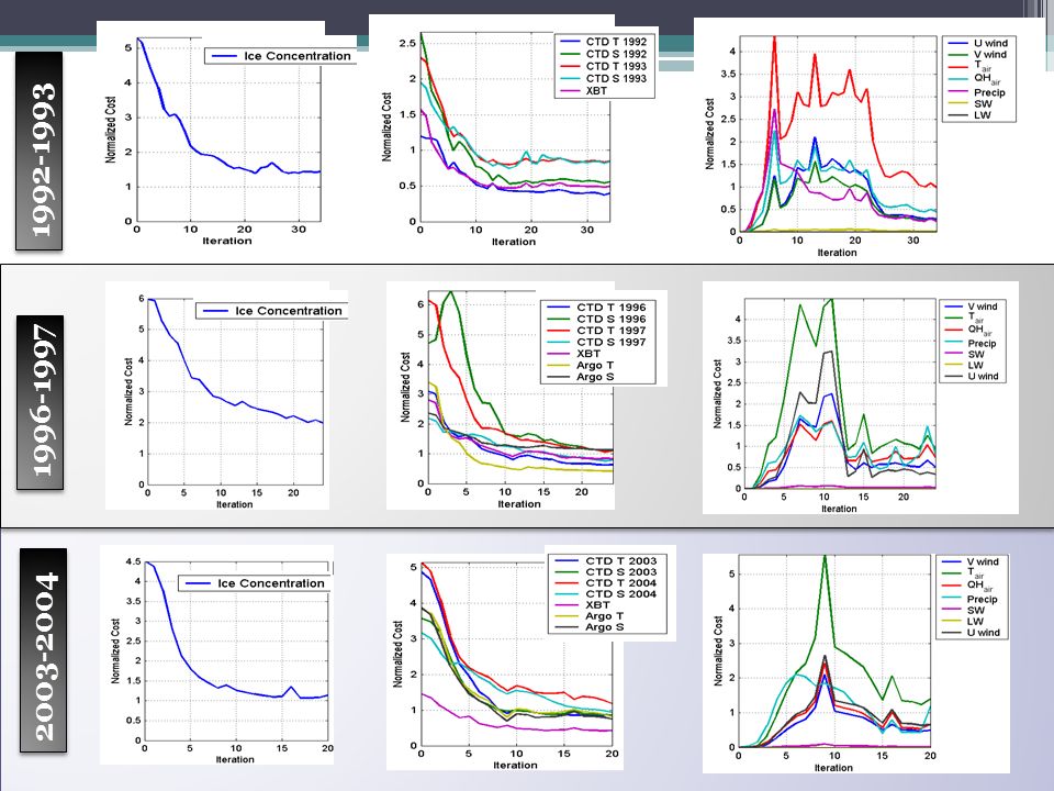
17. Iteration 0 Iteration 33

18. Claim 2 By modifying the sea ice cover these adjustments significantly affect air-sea fluxes

19. Mean and Total Heat Flux Differences March 10, 1993 Annual Mean 92-93

20. Claim 3 Using the adjoint method to synthesize model and observations can reveal systematic errors and biases with both

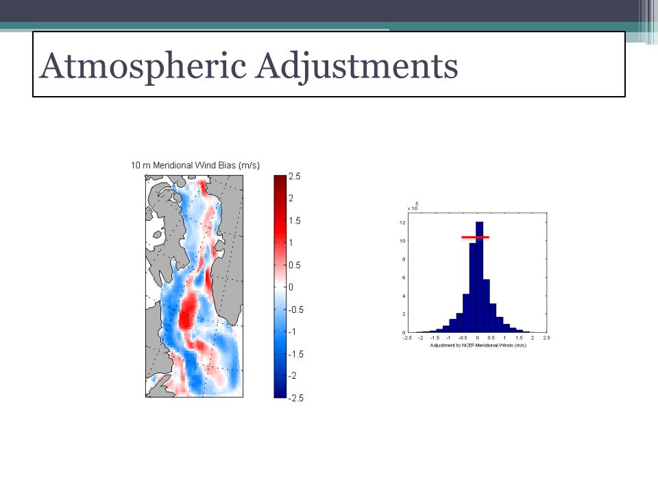
21. Atmospheric Adjustments

23. Conclusions The same model is shown to evolve quite differently based on reasonable adjustments to initial conditions and boundary forcing. Given the known model sensitivity to small changes to atmospheric forcing is there any information in the mean bias atmospheric adjustments that have utility beyond this specific model? ▫AOMIP participants could check this when basin-wide adjustments have been could be disseminated.

24. End

25. Credit Provided by the SeaWiFS Project, NASA/Goddard Space Flight Center, and ORBIMAGE MODIS : May 9, 1999SSM/I : May 9, 1999 6/13/2016 25

26. Thoughts about sea ice data assimilation Data sets ▫Prescribed or assimilated Atmospheric ▫Trustworthiness of renanalyses in high latitudes. ▫Validation in lower latitudes ▫Uncertainties not provided Choice of ocean state ▫Almost certainly the biggest unknown ▫Under many conditions direct assimilation of sea ice state is incompatible with ocean heat content/stratification Sea Ice ▫Different algorithms perform better under different ice conditions ▫Uncertainties are certainly time and space dependent ▫Not provided Formulation of sea ice model ▫Not obvious that more sophisticated sea ice models’ adjoints will be useful Care of interpretation of adjustments ▫Model error is often overlooked ▫Atmospheric controls

27. Interpretation of Atm Controls State Estimate deficiencies ▫Too warm WGC Model deficiency: No boundary current eddies & Mixing ▫ATM wind control ▫Ekman transport of LS surface waters to LC ice edge ▫Increase the gradient so that GM can operate Model deficiency: Ice moves too easily off LC ▫ATM air temp control cools and forms more ice NCEP deficiencies ▫Low resolution, poor location of sea ice edge ▫ATM temp control ▫Warming of off-ice air temp