1. Critical points of the Earth System (Source: H. J. Shellnhuber, IGBP)

2.  How Amazonia functions currently as a regional entity?

3. Vegetation-Climate Interactions Climate Vegetation Bidirectional on what times scales?

4. Nobre et al. 1991, J. Climate Modeling Deforestation and Biogeography in Amazonia Current Biomas Post-deforestation

5. . Avissar et al 2002 Conceptual models of regional deforestation in Amazonia

6. Climate Equilibrium States Oyama, 2002 Vegetation = f (climate) Climate = f (vegetation)

7. A Potential Biome Model that uses 5 climate parameters to represent the (SiB) biome classification was developed (CPTEC-PBM). CPTEC-PBM is able to represent quite well the world’s biome distribution. A dynamical vegetation model was constructed by coupling CPTEC-PBM to the CPTEC Atmospheric GCM (CPTEC-DBM).

8. Five climate parameters drive the potential vegetation model Monthly values of precipitation and temperature Oyama and Nobre, 2002

9. Figure 6. Environmental variables used in CPTEC PVM: growing degree-days on 0 o C base (a), growing degree-days on 5 o C base (b), mean temperature of the coldest month (c), wetness index (d), seasonality index (e). Growing degree-days in oC day month -1, and temperature in o C. growing degree-days on 5 o C base Oyama and Nobre growing degree-days on 0 o C base

10. Wetness index mean temperature of the coldest month Oyama and Nobre

11. seasonality index

12. The potential vegetation model algorithm Oyama and Nobre, 2002 Tropical Forest

13. Visual Comparison of CPTEC-PBM versus Natural Vegetation Map Oyama and Nobre, 2002 CPTEC-PBM SiB Biome Classification

14. Visual Comparison of CPTEC-PBM versus Natural Vegetation Map Oyama and Nobre, 2002 SiB Biome Classification NATURAL VEGETATION POTENTIAL VEGETATION

15. Statistic  (Monserud e Leemans 1992) good agreement poor agreement Oyama and Nobre, 2002 agrement perfect excel. v. good good regular poor v.poor none

16. Objective verification of CPTEC-PBM Oyama and Nobre, 2002 Global Mean Good Very Good Good Very Good Regular Poor Regular agreement

17. Multiple Vegetation-Climate Equilibrium States Oyama, 2002

18. Results of CPTEC-DBM for two different Initial Conditons: all land areas covered by desert (a) and forest (b) Oyama, 2002 Biome-climate equilibrium solution with IC as forest (a) is similar to current natural vegetation (c); when the IC is desert (b), the final equilibrium solution is different for Tropical South America a b c Initial Conditions

19. Oyama and Nobre, 2003 Two Biome-Climate Equilibrium States found for South America!

20. Application of CPTEC-PBM for Past Climate Changes Oyama, 2002 ac (a) PBM results with uniform cooling of 6 C and drying of 3 mm/day to emulate climate conditions of the LGM (21 ka BP); (b) vegetation reconstruction for LGM; (c) PBM results with a uniform cooling of 4 C and rainfall patters with less seasonality over Northeast Brazil; (d) suggestion of pathways for connection of Amazon and Atlantic tropical forests 12-9 ka BP. b d

21. Application of the Potential Vegetation Model (CPTEC- PBM) for Scenarios of Future Climate Change from two Global Climate Models (GCM) Oyama, 2002 CPTEC-PBM GCM scenarios for 2100 Current Potential Vegetation

22. Oyama and Nobre, 2003 Equilíbrios múltiplos bioma-clima para Sahel

23. Possible stability landscape for Tropical South America. Valleys (X1, X2 and Y) and hills correspond to stable and unstable equilibrium states, respectively. Arrows represent climate state (depicted as a black circle) perturbations. State X1 refers to present-day stable equilibrium. For small (large) excursions from X1, state X2 (Y) can be found. It is suggested that the new alternative stable equilibrium state found in this work corresponds to X2. Notice that it is necessary to reach X2 before reaching state Y.

24. Conclusions A Potential Vegetation Model (CPTEC-PVM) was developed that matches quite well the current distribution of biomes in South America; it can be used in a number of applications. Application of CPTEC-PBM to the LGM (21 ka BP) indicates that the rainfall could have been lower by 2-3 mm/day in comparison to present-day values, with considerable dryness throughout the La Plata Basin. For future climates, there might be a slight expansion of subtropical forests into the La Plata Basin. A second biome-climate equilibrium was found for current climate conditions; it shows a northward expansion of the Atlantic forests into the upper reaches of the La Plata Basin

25. Aplications for Past and Future Climates

26. Oyama, 2002 Current Potential Vegetation CSIRO Mk 2 HADC M3 Biome scenarios for 2100

27. Searching for Multiple Biome-Climate Equilibria

28. Climate Equilibrium States Oyama, 2002 P P

29. Figure 1. Potencial (EP) and maximum (Emax) evapotranspiration as function of the temperature for Penman-Monteith (EP and E max ) and Thornthwaite (EP) formulations. Solid line: Thornthwaite, EP; dashed line: Penman-Monteith, E max ; dotted line: Penman- Monteith, EP. Oyama and Nobre

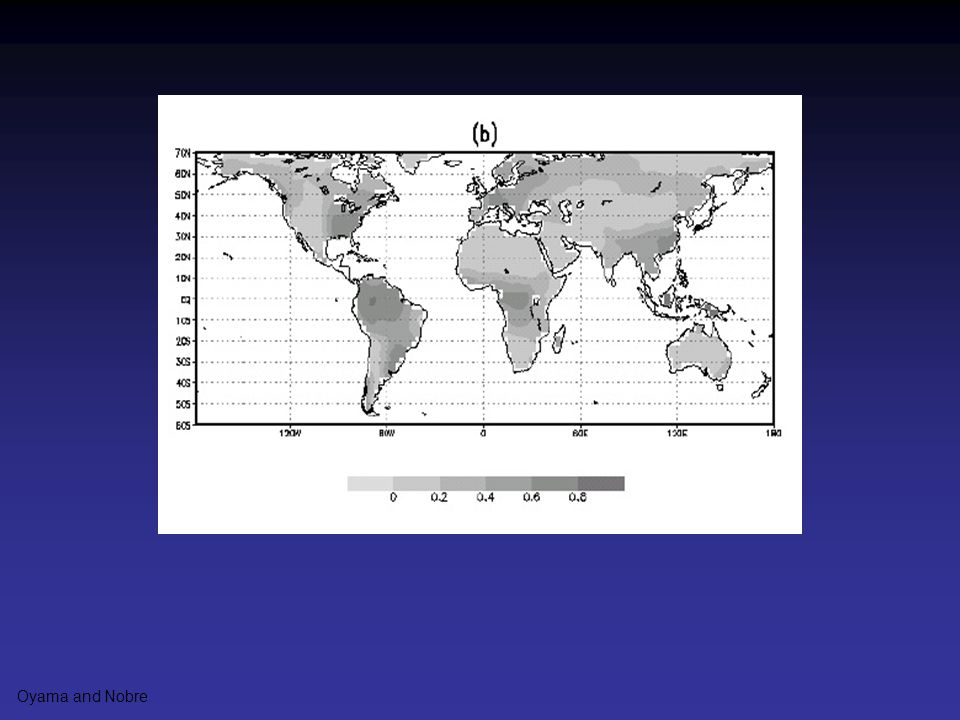
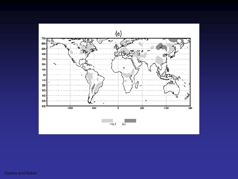
30. Figure 2. Annual average soil water degree of saturation (ratio between soil water storage and soil water availability). (a) Willmott et al. (1985), (b) the present water balance model, and (c) difference between (a) and (b). Oyama and Nobre

33. Figure 3. Annual average soil water degree of saturation according to Willmott et al. (1985, horizontal axis) and the present model (vertical axis). Oyama and Nobre

34. Figure 4. Linear correlation coefficient of the monthly average soil water degree of saturation between Willmott et al. (1985) and the present model results (for all land surfaces between 60 o S and 70 o N). Oyama and Nobre

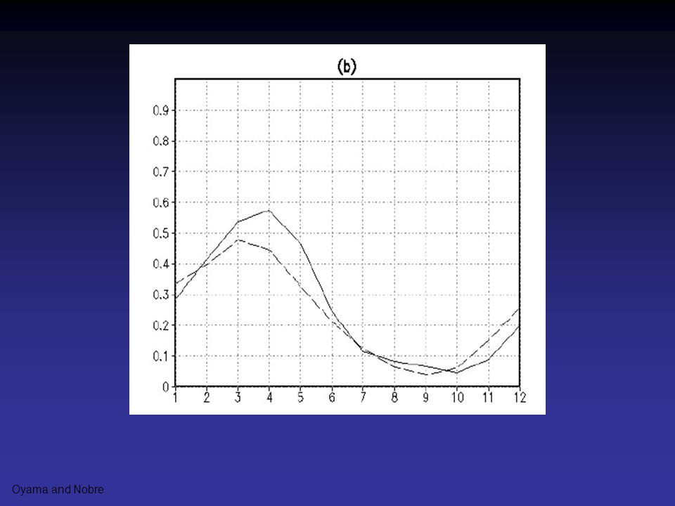
35. Figure 5. Soil water degree of saturation according to Willmott et al. (1985; solid lines) and the present model (dashed lines) for: (a) Amazonia (70 o W-50 o W; 10 o S-Equator) and (b) Northeast Brazil (45 o W-40 o W; 15 o S-5 o S). Oyama and Nobre

37. Figure 8. Natural (a) and potential (b) vegetation map (see Table 1 for vegetation types). Oyama and Nobre

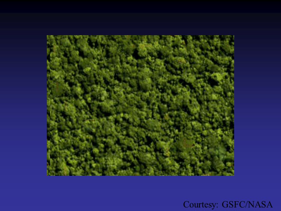
38. Courtesy: GSFC/NASA

40. a b Blow-up for South America: (a) natural vegetation, and (b) biome-climate equilibrium starting from desert land cover as Initial Condition for the Dynamic Vegetation Model. Oyama and Nobre, 2003

41. A Novel Biome-Climate Model: Applications to the Pampa Cruzeiro, SP, Brazil 6-8 Octubre 2003 PROSUR Meeting Centro de Previsão de Tempo e Estudos Climáticos – CPTEC/INPE Marcos Oyama and Carlos A. Nobre CPTEC/INPE

42. Figure 7. Algorithm used to obtain the potential biome from the environmental variables. Temperatures are given in o C; growing degree-days (G 0, G 5 ), in oC day month -1. Oyama and Nobre