1. Introduction to Computer Simulation of Physical Systems (Lecture 10) Numerical and Monte Carlo Methods (CONTINUED) PHYS 3061

2. Monte Carlo Error Analysis Both the classical numerical integration methods and the Monte Carlo methods yield approximate answers The accuracy depends on – the number of intervals – or on the number of samples.

3. We have used the exact value of various integrals to determine the error – in the Monte Carlo methods, it approaches zero as n −1/2 for large n, where n is the number of samples. In this section, we will learn how to estimate the error when the exact answer is unknown.

4. Our main result : the n −1/2 dependence of the error is general, and it is independent of the nature of the integrand and independent of the number of dimensions.

5. We first determine the error for an explicit example. Consider the Monte Carlo evaluation of the integral of f(x) = 4√(1 − x 2 ) in the interval [0, 1]. Our result for a particular sequence of n = 104 random numbers using the sample mean method is Fn = 3.1489.

6. By comparing Fn to the exact result of F = π ≈ 3.1416, we find that the error associated with n = 10 4 samples is approximately 0.0073. How do we know if n = 10 4 samples is sufficient to achieve the desired accuracy?

7. We cannot answer this question definitively because if the actual error were known, we could correct Fn by the required amount and obtain F. The best we can do – to calculate the probability that the true value F is within a certain range centered about Fn.

11. Because this value of σ is two orders of magnitude larger than the actual error, we conclude that σ is not a direct measure of the error. Another clue to finding an appropriate measure of the error – increasing n and seeing how the actual error decreases as n increases. – In Table 11.2 we see that as n is increased from 10 2 to 10 4, the actual error decreased by a factor of approximately 10, that is, as ∼ 1/n 1/2.

12. We also see that the actual error is approximately given by σ/√n. Examples of Monte Carlo measurements of the mean value of f(x) = 4 √(1 − x 2 ) in the interval [0, 1]. The actual error is given by the difference |Fn − π|.

13. the standard error of the means, σ m, is given by σ m = σ / √ (n − 1)≈ σ/ √ n. The interpretation of σ m : if we make many independent measurements of Fn, each with n data points, then the probable error associated with any single measurement is σ m.

14. The more precise interpretation of σ m : F n, our estimate for the mean, has a 68% chance of being within σ m of the “true” mean, and a 97% chance of being within 2σm. This interpretation assumes a Gaussian distribution of the various measurements.

15. The quantity F n is an estimate of the average value of the data points. As we increase n, the number of data points, we do not expect our estimate of the mean to change much. What changes as we increase n is our confidence in our estimate of the mean. Similar considerations hold – for our estimate of σ, – which is why σ is not a direct measure of the error.

16. The error estimate assumes that the data points are independent of each other. However, in many situations the data is correlated! and we have to be careful about how we estimate the error.

17. For example, suppose that instead of choosing n random values for x, We instead start with a particular value x 0 and then randomly add increments such that the ith value of x is given by xi = xi−1 + (2r − 1)δ, where r is uniformly distributed between 0 and 1 and δ = 0.01. Clearly, the xi are now correlated.

18. We can still obtain an estimate for the integral, but we cannot use σ/√n as the estimate for the error because this estimate would be smaller than the actual error. However, we expect that two data points, xi and xj, will become uncorrelated if |j − i| is sufficiently large.

19. How can we tell when |j − i| is sufficiently large? One way is to group the data by averaging over m data points. We take f (m) 1 to be the average of the first m values of f(x i ), f (m) 2 to be the average of the next m values, and so forth.

20. Then we compute σs/√s, Where s = n/m is the number of f (m) i data points, each of which is an average over m of the original data points, σs is the standard deviation of the s data points, We do this grouping for different values of m (and s) the value of m for which σs/√s becomes approximately independent of m. This ratio is our estimate of the error of the mean.

21. We see that we can make the probable error as small as we wish by either increasing n, The number of data points, or by reducing the variance σ 2. Several reduction of variance methods are introduced in Sections 11.6 and 11.7.

22. Nonuniform Probability Distributions In Sections 11.2 and 11.4, how uniformly distributed random numbers can be used to estimate definite integrals. more efficient to sample the integrand f(x) more often in regions of x where the magnitude of f(x) is large or rapidly varying.

23. Because importance sampling methods require nonuniform probability distributions, we first consider several methods for generating random numbers that are not distributed uniformly. In the following, we will denote r as a member of a uniform random number sequence in the unit interval 0 ≤ r < 1.

24. Suppose that two discrete events 1 and 2 occur with probabilities p1 and p2 such that p1+p2 =1. How to choose the two events with the correct probabilities using a uniform probability distribution?

25. For this simple case, it is clear that we choose event 1 if r < p1; otherwise, we choose event 2. If there are three events with probabilities p1, p2, and p3, then if r < p1 we choose event 1; else if r < p1 + p2, we choose event 2; else we choose event 3.

26. We can visualize these choices by dividing a line segment of unit length into three pieces

27. Now consider n discrete events. How do we determine which event, i, to choose given the value of r? The generalization of the procedure we have followed for n = 2 and 3 is to find the value of i that satisfies the condition where we have defined p0 ≡ 0.

28. Now consider a continuous nonuniform probability distribution. to take the limit of the above equation and associate pi with p(x)Δx, where the probability density p(x) is defined such that p(x)Δx is the probability that the event x is in the interval between x and x + Δx. The probability density p(x) is normalized such that

29. In the continuum limit the two sums become the same integral and the inequalities become equalities. Hence we can write we see that the uniform random number r corresponds to the cumulative probability distribution function P(x), which is the probability of choosing a value less than or equal to x.

30. The function P(x) should not be confused with the probability density p(x) or the probability p(x)Δx. In many applications the meaningful range of values of x is positive. In that case, we have p(x) = 0 for x < 0.

31. the inverse transform method for generating random numbers distributed according to the function p(x). This method involves generating a random number r and solving (11.30) for the corresponding value of x. As an example of the method, we use (11.30) to generate a random number sequence according to the uniform probability distribution on the interval a ≤ x ≤ b. The desired probability density p(x) is p(x) =1/(b − a) a ≤ x ≤ b; 0, otherwise

32. The cumulative probability distribution function P(x) for a ≤ x ≤ b : P(x) =(x − a)/(b − a). If we solve for x, the desired relation is: x = a + (b − a)r. The variable x is distributed according to the probability distribution p(x).

33. We next apply the inverse transform method to the probability density function If we substitute (11.34) into (11.30) and integrate, we find the relation r = P(x) = 1 − e −x/λ. (11.35)

34. The solution of (11.35) for x yields x = −λ ln(1−r). Because 1−r is distributed in the same way as r, we can write x = −λ ln r. (11.36) The variable x found from (11.36) is distributed according to the probability density p(x) given by (11.34). Because the computation of the natural logarithm in (11.36) is relatively slow, the inverse transform method might not be the most efficient method to use in this case.

35. From the above examples, two conditions must be satisfied in order to apply the inverse transform method: the form of p(x) must allow us to perform the integral in (11.30) analytically, and it must be practical to invert the relation P(x) = r for x.

36. The Gaussian probability density, p(x) =[1/(2πσ2) 1/2 ]e −x^2/2σ^2, (11.37) is an example of a probability density for which the cumulative distribution P(x) cannot be obtained analytically. However, we can generate the two- dimensional probability p(x, y) dx dy given by p(x, y) dx dy = (1/2πσ 2 )e −(x^2+y^2)/2σ^2 dx dy.

37. First, we make a change of variables to polar coordinates: r = (x 2 + y 2 ) 1/2, θ = tan −1 y/x. (11.39) We let ρ = r 2 /2 and write the two-dimensional probability as p(ρ, θ) dρ dθ =(1/2π)e −ρ dρ dθ, (11.40) where we have set σ = 1.

38. If we generate ρ according to the exponential distribution (11.34) and generate θ uniformly in the interval 0 ≤ θ < 2π, then the quantities x = (2ρ) 1/2 cos θ and y = (2ρ) 1/2 sin θ (Box-Muller method) will each be generated according to (11.37) with zero mean and σ = 1. (Note that the two dimensional density (11.38) is the product of two independent one-dimensional Gaussian distributions.) This way of generating a Gaussian distribution is known as the Box-Muller method.

39. Importance Sampling In Section 11.4 we found that the error associated with a Monte Carlo estimate is proportional to the standard deviation σ of the integrand and inversely proportional to the square root of the number of samples.

40. Hence, there are only two ways of reducing the error in a Monte Carlo estimate – either increase the number of samples or reduce the variance. Clearly the latter choice is desirable because it does not require much more computer time. In this section we introduce importance sampling techniques that reduce σ and improve the efficiency of each sample.

41. To do importance sampling in the context of numerical integration, we introduce a positive function p(x) such that ∫ b a p(x) dx = 1, (11.43) and rewrite the integral (11.1) as F =∫ b a [f(x)/p(x)] p(x) dx.(11.44)

42. We can evaluate the integral (11.44) by sampling according to the probability distribution p(x) and constructing the sum Fn =1/nΣf(xi)/p(xi). i= 1 to n, (11.45) The sum (11.45) reduces to (11.15) for the uniform case p(x) = 1/(b − a).

43. The idea is to choose a form for p(x) that minimizes the variance of the ratio f(x)/p(x). To do so we choose a form of p(x) that mimics f(x) as much as possible, particularly where f(x) is large. A suitable choice of p(x) would make the integrand f(x)/p(x) slowly varying, and hence reduce the variance.

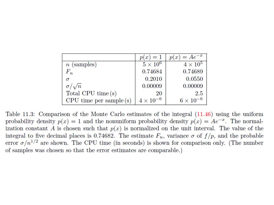
44. Because we cannot evaluate the variance analytically in general, we determine σ a posteriori. As an example, we consider the integral F =∫ 1 0 exp (−x 2 )dx. The estimate of F with p(x) = 1 for 0 ≤ x ≤ 1 is shown in the second column of Table 11.3. A simple choice for the weight function is p(x) = Ae −x, where A is chosen such that p(x) is normalized on the unit interval.

46. Note that this choice of p(x) is positive definite and is qualitatively similar to f(x). The results are shown in the third column of Table 11.3. We see that although the computation time per sample for the non-uniform case is larger, the smaller value of σ makes the use of the non-uniform probability distribution more efficient.

47. Metropolis Algorithm Another way of generating an arbitrary nonuniform probability distribution was introduced by Metropolis, Rosenbluth, Rosenbluth, and Teller in 1953. The Metropolis algorithm is a special case of an importance sampling procedure in which certain possible sampling attempts are rejected (see Appendix 11C).

48. The Metropolis method is useful for computing averages of the form f =∫f(x)p(x) dx/[ ∫p(x) dx], (11.52) where p(x) is an arbitrary function that need not be normalized. For simplicity, we introduce the Metropolis algorithm – in the context of estimating one-dimensional definite integrals. Suppose that we wish to use importance sampling to generate random variables according to p(x).

49. The Metropolis algorithm produces a random walk of points {xi} – whose asymptotic probability distribution approaches p(x) after a large number of steps. The random walk is defined by specifying a transition probability T(x i → x j ) from one value x i to another value x j such that the distribution of points x 0, x 1, x 2,... converges to p(x). It can be shown that it is sufficient (but not necessary) to satisfy the detailed balance condition p(xi)T(xi → xj) = p(xj)T(xj → xi). (11.53) – We’ll give the detailed proof in PHYS4370.

50. The relation (11.53) does not specify T(x i → x j ) uniquely. A simple choice of T(x i → x j ) that is consistent with (11.53) is T(x i → x j ) = min[1,p(x j )/p(x i )]. (11.54) If the “walker” is at position x i and we wish to generate x i+1, we can implement this choice of T(x i → x i+1 ) by the following steps:

51. 1. Choose a trial position x trial = x i + δ i, – where δi is a uniform random number in the interval [−δ, δ]. 2. Calculate w = p(x trial )/p(xi). 3. If w ≥ 1, accept the change and let x i+1 = x trial. 4. If w < 1, generate a random number r. 5. If r ≤ w, accept the change and let x i+1 = x trial. 6. If the trial change is not accepted, then let x i+1 = x i.

52. It is necessary to sample many points of the random walk before the asymptotic probability distribution p(x) is attained. How do we choose the maximum step size δ? If δ is too large, only a small percentage of trial steps will be accepted and the sampling of p(x) will be inefficient. On the other hand, if δ is too small, a large percentage of trial steps will be accepted, but again the sampling of p(x) will be inefficient.

53. A rough criterion for the magnitude of δ is that approximately one third to one half of the trial steps should be accepted. We also wish to choose the value of x 0 – such that the distribution {xi} will approach the asymptotic distribution as quickly as possible. An obvious choice is to begin the random walk at a value of x at which p(x) is a maximum. A code fragment that implements the Metropolis algorithm is given below.

54. Read neutron transport section if you are interested. double xtrial = x + (2* rnd.nextDouble ( ) - 1.0 ) * delta; double w = p( xtrial )/p( x ) ; i f (w > 1 || w > rnd.nextDouble ( ) ) { x = xtrial ; naccept++; // number of acceptances }

55. Error Estimates for Numerical Integration We derive the dependence of the truncation error on the number of intervals for the numerical integration methods considered in Sections 11.1 and 11.3. These estimates are based on the assumed adequacy of the Taylor series expansion of the integrand f(x): f(x) = f(xi) + f′(xi)(x − xi) +1/2f′′(xi)(x − xi)2 +..., (11.64)

56. and the integration of (11.1) in the interval xi ≤ x ≤ xi+1: ∫ xi+1 xi f(x) dx = f(xi)Δx +1/2f′(xi)(Δx) 2 +1/6f′′(xi)(Δx) 3 +... (11.65) We first estimate the error associated with the rectangular approximation with f(x) evaluated at the left side of each interval.

57. The error Δi in the interval [xi, xi+1] is the difference between (11.65) and the estimate f(xi)Δx: Δi =[∫ xi+1 xi f(x) dx]− f(xi)Δx ≈ 1/2f′(xi)(Δx) 2. (11.66) We see that to leading order in Δx, the error in each interval is order (Δx) 2. Because there are a total of n intervals and Δx = (b − a)/n, the total error associated with the rectangular approximation is nΔ i ∼ n(Δx) 2 ∼ n −1.

58. The estimated error associated with the trapezoidal approximation can be found in the same way. The error in the interval [xi, xi+1] is the difference between the exact integral and the estimate, 1/2 [f(xi) + f(xi+1)]Δx: Δ i =[ ∫ xi+1 xi f(x) dx]− ½ [f(xi) + f(xi+1)]Δx. (11.67)

59. If we use (11.65) to estimate the integral and (11.64) to estimate f(xi+1) in (11.67), we find that the term proportional to f′ cancels and that the error associated with one interval is order (Δx) 3. Hence, the total error in the interval [a, b] associated with the trapezoidal approximation is order n −2.

60. Because Simpson’s rule is based on fitting f(x) in the interval [xi−1, xi+1] to a parabola, error terms proportional to f′′ cancel. We might expect that error terms of order f′′′(xi)(Δx) 4 contribute, but these terms cancel by virtue of their symmetry.

61. Hence the (Δx) 4 term of the Taylor expansion of f(x) is adequately represented by Simpson’s rule. If we retain the (Δx) 4 term in the Taylor series of f(x), we find that the error in the interval [xi, xi+1] is of order f′′′′(xi)(Δx) 5 and that the total error in the interval [a, b] associated with Simpson’s rule is O(n −4 ).

62. The error estimates can be extended to two dimensions in a similar manner. The two dimensional integral of f(x, y) is the volume under the surface determined by f(x, y). In the “rectangular” approximation, the integral is written as a sum of the volumes of parallelograms – with cross sectional area ΔxΔy – and a height determined by f(x, y) at one corner.

63. To determine the error, we expand f(x, y) in a Taylor series f(x, y) = f(x i, y i ) +(∂f(xi, y i )/∂x) (x − xi) + (∂f(xi, yi) /∂y) (y − yi) +..., (11.68) and write the error as Δi =[∫ ∫f(x, y) dxdy]− f(x i, y i )ΔxΔy. (11.69)

64. If we substitute (11.68) into (11.69) and integrate each term, we find that the term proportional to f cancels and the integral of (x − x i ) dx yields 1/2(Δx) 2. The integral of this term with respect to dy gives another factor of Δy. The integral of the term proportional to (y −y i ) yields a similar contribution.

65. Because Δy also is order Δx, the error associated with the intervals [xi, xi+1] and [yi, yi+1] is to leading order in Δx: Δi ≈ 1/2[f′x(xi, yi) + f′y(xi, yi)](Δx) 3. (11.70) We see that the error associated with one parallelogram is order (Δx) 3. Because there are n parallelograms, the total error is order n(Δx) 3. However in two dimensions, n = A/(Δx) 2, And hence the total error is order n −1/2. In contrast, the total error in one dimension is order n−1.

66. The corresponding error estimates for the two- dimensional generalizations of the trapezoidal approximation and Simpson’s rule are order n −1 and n −2 respectively. In general, if the error goes as order n −a in one dimension, then the error in d dimensions goes as n −a/d. In contrast, Monte Carlo errors vary as n −1/2 independent of d. Hence for large enough d, Monte Carlo integration methods will lead to smaller errors for the same choice of n.