1. The Practice of Statistics Third Edition Daniel S. Yates Chapter 13: Comparing Two Population Parameters Copyright © 2008 by W. H. Freeman & Company

2. Chapter Objectives Identify the conditions needed to do inference for comparing two population means or proportions. Perform a significance test for the difference of two population means or proportions. Construct a confidence interval for the difference between two population means or proportions.

3. Two-Sample Problems Comparing two populations or two treatments is one of the most common situations encountered in statistical practice. Unlike the matched pairs designs, there is no matching of the units in the two samples. The two samples can be different sizes.

4. 13.1 – Comparing Two Means

5. Notation ParametersStatistics PopulationVariableMean Standard Deviation Sample sizeMean Standard Deviation 1x1x1 µ1µ1 σ1σ1 n1n1 s1s1 2x2x2 µ2µ2 σ2σ2 n2n2 s2s2 There are 4 unknown parameters, the two means and the two standard deviations. We want to compare the two population means, either by giving a confidence interval for their difference µ 1 - µ 2 or by testing the hypothesis of no difference, H 0 : µ 1 = µ 2 or H 0 : µ 1 - µ 2 = 0

6. The Two-Sample z Statistic The mean of is µ1 - µ2. The difference of sample means is an unbiased estimator of the difference of population means. The variance of the differences is the sum of the variances of which is Note: variances add, not standard deviations If the population distributions are both Normal, then the distribution of is also Normal

7. When the statistic has a Normal distribution, we can standardize it to obtain a standard Normal z distribution. It is very rare that we would know both population standard deviations, so we would have to use the t procedures.

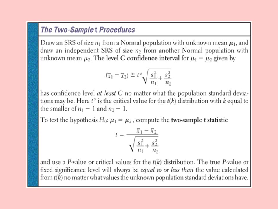
8. The Two-Sample t Procedures The standard error, or estimated standard deviation is When we standardize our estimate ( ), the result is the two- sample t statistic.

9. The Two-Sample t Procedures The two-sample t statistic has approximately a t distribution. It does not have exactly a t distribution even if the populations are both exactly Normal. The approximation, however, is very accurate. The catch is calculating the degrees of freedom….it can be messy.

10. Calculating degrees of freedom There are three options: 1.Use technology to calculate degrees of freedom 2.If n 1 = n 2, then df = n 1 + n 2 – 2 3.Df = the smaller of n 1 – 1 and n 2 – 1. This is a very conservative method. There is a much more complicated method to calculate the degrees of freedom by hand. Most statistical software programs use this method (built into their program)

12. These two-sample procedures always err on the safe side. They report higher P-values and lower confidence than may actually be true. The gap between what is reported and the truth is quite small –Unless the sample sizes are both small and unequal As the sample sizes increase, probability values based on t with degrees of freedom equal to the smaller of n 1 – 1 and n 2 – 1 become more accurate.

13. Example. Calcium and blood pressure. Does increasing the amount of calcium in our diet reduce blood pressure? Examination of a large sample of people revealed a relationship between calcium intake and blood pressure. The relationship was strongest for black men. Such observational studies do not establish causation. Researchers therefore designed a randomized comparative experiment. The subjects in part of the experiment were 21 healthy black men. A randomly chosen group of 11 men received a placebo pill that looked identical. The experiment was double-blind. The response variable is the decrease in systolic (top number) blood pressure for a subject after 12 weeks, in millimeters of mercury. An increase appears as a negative response.

14. Take Group 1 to be the calcium group and Group 2 the placebo group. Group 1 Group 2 From the data, calculate the summary statistics: 7-41817-3-511011-2 12-33-552-11-3 GroupTreatmentns 1Calcium105.0008.743 2Placebo11-0.2735.901

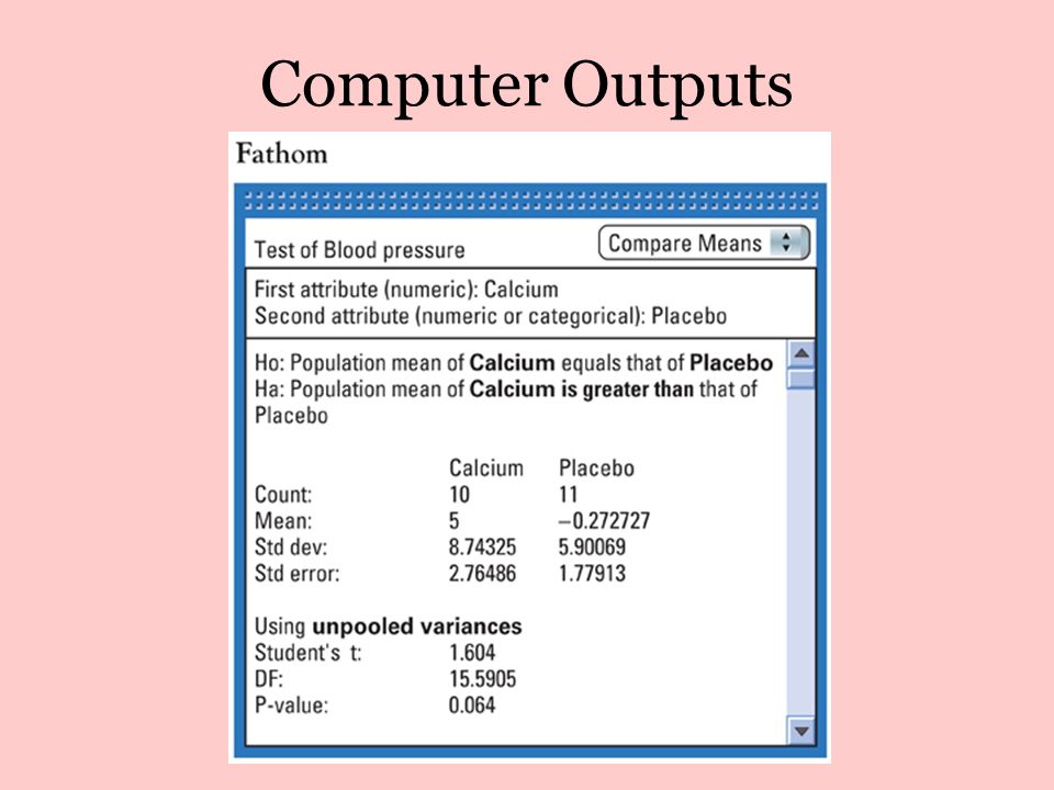
15. The calcium group shows a drop in blood pressure, = 5.000, while the placebo group shows a small increase, = -0.273. Is this outcome good evidence that calcium decreases blood pressure in the entire population of healthy black men more than a placebo does? Step 1: Hypotheses. H 0 : µ 1 = µ 2 H 0 : µ 1 - µ 2 = 0 or H a :µ 1 > µ 2 H a : µ 1 - µ 2 > 0 H 0 : There is no difference in blood pressure between the two treatments H a :The calcium treatment shows a decrease in blood pressure.

16. Step 2: Conditions. SRS – The 21 subjects were not obtained by random selection from a larger population. As a result, it may be difficult to generalize our findings to all healthy black men. However, the random assignment of subjects to treatments should help ensure that any significant difference in mean blood pressure between the two groups is due to the treatment. Independence – Because of the randomization, the calcium group and the placebo group are two independent samples. We cannot use the 10n ≤ N here because we are not sampling from different populations. Normality – We must check for serious non-Normality (outliers). We will use a Normal probability plot.

17. Although the calcium group shows a slightly irregular distribution, there are no outliers. We should feel comfortable using t procedures because they are robust against non-Normality.

18. Step 3: Calculations. Test statistic. The two-sample t statistic is P-value. Df = 9 tcdf(1.604, 1000, 9) = 0.0716

19. Step 4: Interpretation. The experiment provided some evidence that calcium reduces blood pressure, but the evidence falls short of the traditional 5% and 1% levels. We would fail to reject H 0 at either of these significance levels. We can estimate the difference in the mean decrease in blood pressure for the hypothetical calcium and placebo populations using a two- sample t interval.

20. For a 90% confidence interval, and df = 9, t* = 1.833. We are 90% confident that the mean advantage of calcium over placebo, u 1 – u 2 lies between -0.0753 and 11.299 Since the 90% confidence interval includes 0, we would fail to reject H 0 : u 1 – u 2 = 0 against the two-sided alternative at the α = 0.10 level of significance. HW: pg. 785 #13,1, 13.2, 13.5 / pg. 791 #13.7, 13.9 (goes with 13.5)

21. Software Approximation for the Degrees of Freedom Note: The degrees of freedom do not have to be a whole number.

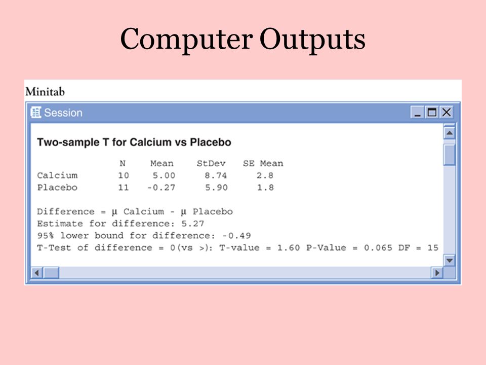
22. Calcium and blood pressure continued…….. Here is the data summary again. GroupTreatmentns 1Calcium105.0008.743 2Placebo11-0.2735.901

23. Computer Outputs

26. Using your Graphing Calculator for a Two-Sample T Test Enter data for calcium group in L1 and placebo group in L2. Go to STAT/TESTS and choose 4: 2-SampTTest In the 2-SampTTest screen, specify “Data” and adjust your inequality to match your alternative hypothesis. Arrow down and highlight “Calculate” and press ENTER. –Always pick “No” for pooling If you pick “Draw” the t(k) distribution will be displayed. –It will only display the t test statistic and the p-value.

27. Using your Graphing Calculator for a Two-Sample T Interval Enter data for calcium group in L1 and placebo group in L2. Go to STAT/TESTS and choose 2-SampTInt In the 2-SampTTest screen, specify “Data” and desired level of confidence Arrow down and highlight “Calculate” and press ENTER. –Always pick “No” for pooling If you are given a data summary instead of actual data values, select the “Stats” option instead. Then provide the values requested.

28. Example. DDT poisoning. Poisoning by the pesticide DDT causes convulsions in humans and other mammals. Researchers seek to understand how the convulsions are caused. In a randomized comparative experiment, they compared 6 white rats poisoned with DDT with a control group of 6 unpoisoned rats. Electrical measurements of nerve activity are the main clue to the nature of DDT poisoning. When a nerve is stimulated, its electrical response shows a sharp spike followed by a much smaller second spike. The experiment found that the second spike is larger in rats fed DDT than in normal rats. This finding helped biologists understand how DDT poisoning works.

29. The researchers measured the height of the second spike as a percent of the first spike when a nerve in the rat’s leg was stimulated. For the poisoned rats the results were The control group data were 12.20716.86925.05022.4298.45620.589 11.0749.68612.0649.3518.1826.642

30. Researchers didn’t conjecture in advance that the size of the second spike would be higher in rats fed DDT, they only conjectured that it would be different. Step 1: Hypotheses. H 0 : µ DDT = µ NORMAL H a : µ DDT ≠ µ NORMAL

31. Step 2: Conditions. SRS – The researchers used a randomized comparative experiment. The rats were randomly assigned to the two treatments. Independence – Due to the random assignment, the researchers can treat the two groups of rats as independent samples. Normality – Normal probability plots show no outliers.

32. Step 3: Calculations. Use your calculator to determine the missing values. = 17.6 = 9.4998 s 1 = 6.340s 2 = 1.945 t = 2.9912p-value = 0.0246 df = 5.938

33. Step 4: Interpretation. The low P-value provides strong evidence against the null. We can reject H o at the 5% significance level. We conclude that the mean size of the secondary spike is larger in rats fed DDT. HW: pg. 801 #13.13, 13.16

34. 13.2 – Comparing Two Proportions Population proportion Sample size Sample proportion 1p1p1 n1n1 2p2p2 n2n2 We do inference about the difference p1 – p2 between the population proportions to compare the populations. The statistic that estimates this difference is the difference between the sample proportions,

35. The Sampling Distribution of Center: the mean of is Spread: The standard deviation of is Shape: When the samples are large, the distribution of is approximately Normal. –This will happen if n 1 (p 1 ), n 1 (1 - p 1 ), n 2 (p 2 ), and n 2 (1 - p 2 ) are all ≥ 10.

36. The Sampling Distribution of

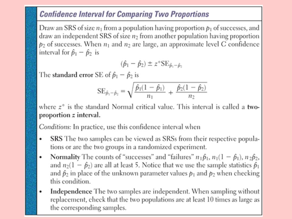
37. Confidence Intervals for To obtain a confidence interval, replace the population proportions p 1 and p 2 with the sample proportions. The result is the standard error. The confidence interval again has the form estimate ± z*SE estimate

39. Example. How much does preschool help? To study the long term effects of preschool programs for poor children, the High/Scope Educational Research Foundation has followed two groups of Michigan children since early childhood. A control groups of 61 children represents Population 1, poor children with no preschool. Another group of 62 children from the same area and similar backgrounds attended preschool as 3- and 4-year-olds. This is a sample from Population 2, poor children who attend preschool. The response variable of interest is the need for social services as adults. In the past 10 years, 38 of the preschool sample and 49 of the control group have needed social services (mainly welfare) Does this study provide significant evidence that preschool reduces the later need for social services?

40. Step 1: Hypotheses. H o : p 1 = p 2 H a : p 1 > p 2 p 1 = proportion of poor children who don’t attend preschool and who need social services as adults p 2 = proportion of poor children who attend preschool and who need social services as adults. We will start by calculating a two-proportion z interval.

41. Step 2: Conditions SRS: We are not told how the two samples were selected. We must use caution when drawing conclusions about the corresponding population. Normality: –These are all at least 5, so the interval based on Normal calculations will be reasonably accurate. Independence: We can be fairly confident that there are at least 610 poor children who did not attend preschool and 620 poor children who did in our population of interest.

42. Step 3: Calculations. To compute a 95% confidence interval first calculate the standard error. The 95% confidence interval is

43. Computer Outputs

44. Step 4: Interpretation. We are 95% confident that the percent needing social services is somewhere between 3.3% and 34.7% lower among people who attended preschool. The confidence interval is wide because the sample sizes are a bit small for estimating an unknown proportion with precision. The researchers selected two separate samples from the two populations they wanted to compare. Many comparative studies start with just one sample, the divide it into two groups based on data gathered from the subjects. The two-proportion z procedures are valid in such situations. HW: pg. 813 #13.27

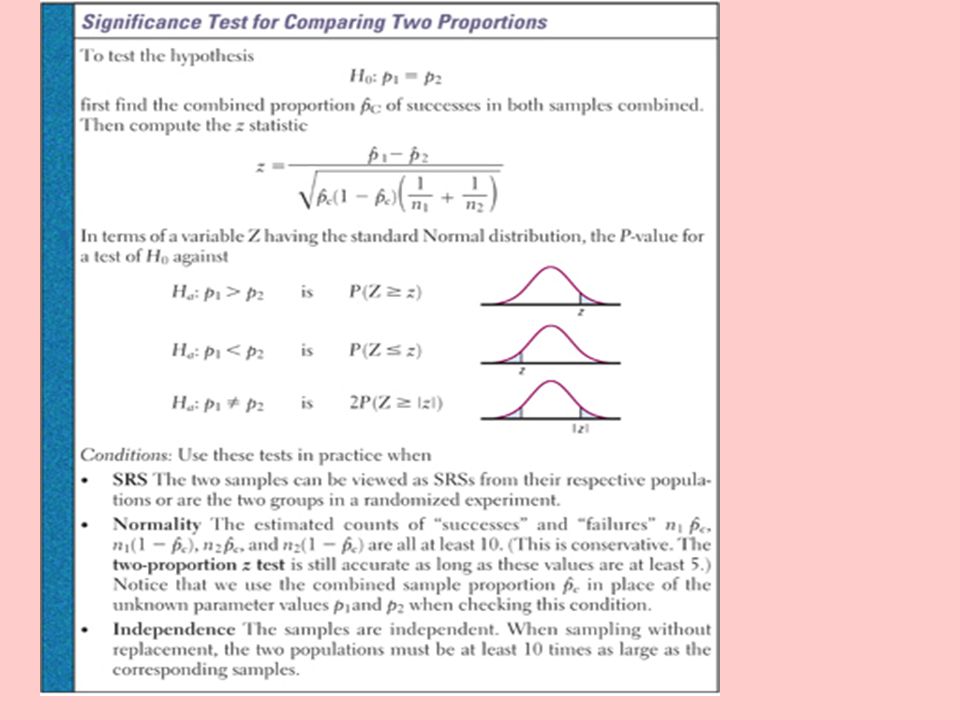
45. Significance Tests for p 1 – p 2 The null hypothesis says that there is no difference between the two populations: H 0 : p 1 = p 2 The alternative hypothesis says what kind of difference we expect. Checking Normality: must all be at least 10. The test statistic formula uses the combined sample proportion.

47. Notice how this formula is different than the SE for confidence intervals. has replaced both and in the formula When checking normality you can check that are all greater than 10 (some books use 5)

48. Example. How much does preschool help? continued… Recall our H 0 : p 1 = p 2 and H a : p 1 > p 2 Population DescriptionSample Size Number needing social services 1Control6149 2Preschool6238

49. Check Normality condition.

50. Calculations P-value: P(z > 2.31) = P(z < -2.31) = 0.0104

51. Interpretation. Our P-value, 0.0104, tells us that it is unlikely that we would obtain a difference in sample proportions as large as we did if the null hypothesis is true. Since our P-value is less than 0.05, we can reject H 0. We can conclude poor children who did not attend preschool are more likely to need social services than poor children who did attend preschool.

52. Using your Graphing Calculator for a Two-Proportion Z Test Go to STAT/TESTS and choose 6: 2-PropZTest In the 2-PropZTest screen, enter x 1, n 1, x 2, n 2 and adjust your inequality to match your alternative hypothesis. –Where x 1 and x 2 represent the successes for the samples. Arrow down and highlight “Calculate” and press ENTER. If you pick “Draw” the z distribution will be displayed. –It will only display the z test statistic and the p-value. Now try it on Example 13.42 on pg. 828. HW: pg. 819 #13.30