1. INSTRUMENTAL VARIABLES Eva Hromádková, 4.11.2010 Applied Econometrics JEM007, IES Lecture 5

2. Reminder Basic issue in causal inference: Observed correlation between X (treatment) and Y (outcome) (X ~Y) does not imply causal relationship X=> Y  Simultaneity: X  Y (example: supply x demand)  Endogeneity: W=>X & W=>Y => (X ~Y) To find whether there exist causal relationship (“treatment effect”), we need to find identification strategy  Some method that will “distill” the effect of X on Y

3. Instrumental variables Intuition  Treatment status is predicted by some other variable (instrumental variable), that is otherwise not related with the outcome variable 2 conditions for instrumental variable Z:  Correlated with treatment X (Monotonicity)  Uncorrelated with any other determinant of the outcome variable Y (Exclusion restriction)  The only way how instrument affects outcome is through X We are only using variance in X that is induced by Z!

4. Instrumental variables Equations On the example of effect of education on wages:  Problem = endogeneity = person’s ability determines both the educational attainment as well as his wage  We need to instrument for education:

5. Instrumental variables Estimation - 2SLS 1 st Stage: Regress the endogenous variable (EDU) on the instrument Z and all other exogenous variables X  Intuition: “distill” variation in EDU that is due to changes (variation) in instrument Z ONLY 2 nd Stage: Regress the outcome variable (ln wage) on the predicted values of EDU and X’s

6. Instrumental variables Estimation - 2SLS  Careful with 2SLS!  β from 2SLS is not unbiased, just consistent  !source of the weak IV problem (if we have even small endogeneity, it is multiplied by weakness)  If we really run 2 regressions – SE will be wrong (Q – why?) ivreg2 does it for us already

7. Instrumental variables Issues 1. Is my instrument really uncorrelated with other determinants of the outcome? 2. How strong does my first stage have to be for this to all work? 3. How do I interpret my IV estimate? What if I think there are heterogeneous treatment effects?

8. Issues in IV: 1. Do I need IV & testing the exclusion restriction Do I need IV?  If we have IV, we can test for endogeneity of suspected variable  Hausman test, Durbin-Wu-Hausman test  H0: suspected variable is exogenous (OLS is prefered) Testing exclusion restriction?  If we have multiple instruments, we can test using the over- identification test  Take one instrument as valid and test whether other instruments are excluded (insignificant) in the second stage  !we have to assume that at least 1 IV is valid!

9. Issues in IV: 2. Problem of weak IV  Bound, Jaeger and Baker (1995) – “the cure can be worse than disease” – if the excluded instruments are only weakly correlated with the endogenous variables  IV estimates will be biased in same direction as OLS  Weak IV estimates may not be consistent  Tests of significance have incorrect size and confidence intervals are wrong  Strong and Young (2005) – “rule of thumb”  Previously, F-stat from first stage >10 + look at partial R2 from the first stage regression  Now – compare F-statistics with Table1/2 from Strong and Young  http://www.stata.com/meeting/5nasug/wiv.pdf

10. Issues in IV: 3. Heterogenous treatment effects I Problem:  Changes in instrumental variable Z drive into treatment people with higher expected gains  Example: as IV for education we use costs of education – e.g. distance to college  Exclusion restriction: proximity to college should not have any effect on wage other than through education  Result: observed distribution of ability of college students is different for low-costs and high costs students  Q1: what differences in distribution would you expect?  Q2: if I randomly assign costs to individuals, do I solve the baseline problem?

11. Issues in IV: 3. Heterogenous treatment effects II LATE – local average treatment effect for IV  We only measure the effect of treatment on the people whose switch from untreated to treated is triggered by the instrumental variable  Ex: our identification strategy identifies the return to education only for the subset of population that is sensitive to costs  The group of “movers” from treated to untreated is not representative of whole population (“local” effect)

12. Issues in IV: 3. Heterogenous treatment effects III LATE – local average treatment effect for IV  Discreet parameter – “policy introduction” used as instrument  LATE will measure the treatment on the subset of population that is sensitive to the policy change (“compliers”)  This can bring insight as to the effectivity of such policy  Continuous characteristics as IV – much less informative

13. Application of IV What was used as an IV?  Geography as an instrument  (distance, rivers, small area variation)  Legal/political institutions as an instrument  (laws, election dynamics)  Administrative rules as an instrument  (wage/staffing rules, reimbursement rules, eligibility rules)  Naturally occurring randomization  (draft, birth date, lottery, roommate assignment, weather)

14. Example 1: Angrist (1990) Introduction Question: effect of serving in Vietnam war on earnings  But, people who choose to serve may be different from people who did not enlist, and this might be correlated with their earnings perspective (Q: how?)  Use of natural experiment = draft lottery number  Random number (RSN) was assigned to each date of birth  Ceiling was set, only men with lottery numbers below ceiling could be drafted (in 70 195, in 72’ 95) – draft eligible  Wi = 1 if person was enlisted (either drafted, or self-enlist)  Zi = 1 if person was eligible for draft

15. Example 1: Angrist (1990) Introduction OLS results: Military status(W) by eligibility (Z)  Compliers (obey assignment)  Always takers  Never takers  Defiers  Q: where can we find who?

16. Example 1: Angrist (1990) Estimates I  Estimated proportions of types:  Ass: there are no defiers  Q: What is wrong with this?  Average log earnings by groups

17. Example 1: Angrist (1990) Estimates III  2SLS – results  Outcomes for compliance groups:

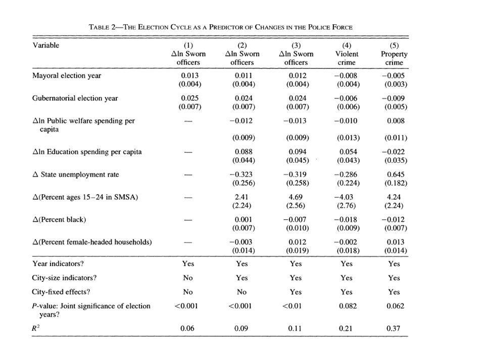
18. Example 2: Levitt (1997)  IV application in the case of simultaneity  Question: does police reduce crime?  BUT more crime => more police  Instrument: increase in the size of police forces during electorial years

19. Example 2: Levitt (1997) Is instrument valid?