1. The Simple Linear Regression Model: Specification and Estimation  Theory suggests many relationships between variables  These relationships suggest that we can: Answer the How Much Questions Forecast or predict the corresponding value of one variable  The SLRM can be used to accomplish these goals.

2. The Simple Linear Regression Model: Specification and Estimation  Suppose that we are interested in studying the relationship between consumption and income.  We can gather data from different households and then analyze it.  But how do we analyze it?

3. The Simple Linear Regression Model: Specification and Estimation  We know that theory suggests that consumption is a function of income (and other variables that for now we will ignore). Therefore our economic model would be something like this:

4. The Simple Linear Regression Model: Specification and Estimation  We are interested in answering questions like: How much will consumption increase if income increases by 10%?  To answer this question we need to assume a functional form for our consumption- income relationship like:

5. The Simple Linear Regression Model: Specification and Estimation  Equation (1) represents our economic model, it shows that as income increases consumption increases.  NOTE: Economic models are not used to predict exact relationships among variables, they predict the average relationship between the variables

6. The Simple Linear Regression Model: Specification and Estimation  We can transform our economic model, equation (1), into an econometric model. We can see that theory suggests a linear relation between C and I. We must account for the fact that our theoretical model needs to be modified in order to include a random disturbances.  Random what?? And why ???

7. The Simple Linear Regression Model: Specification and Estimation  Our econometric model includes the random disturbances and can be expressed as: Non Random Random/stochastic  This is a simple linear regression model. ??

8. The Simple Linear Regression Model: Specification and Estimation  It is important to differentiate the econometric model in equation (2) from two other concepts/analysis that you may be familiar with: Correlation ??? Causation ???

9. The Simple Linear Regression Model: Specification and Estimation  Now that we have a clear idea of what the regression model is all about, we must state and clearly explain the assumptions behind it.

10. The Simple Linear Regression Model: Specification and Estimation  The Assumptions of the SLRM: 1.The dependent variable can be expressed as a linear function of the regressors. 2.The disturbance term has a mean of zero. 3.The variance of the random error/disturbance is: 4.The covariance between any pair of random errors is zero. 5.The variable x (regressor) is not random and must take at least two different values. 6.(optional) The values of e are normally distributed about their mean, if the values of y are normally distributed, and vice versa.

11. The Simple Linear Regression Model: Specification and Estimation  Now the great task at hand is to estimate the values for  1 and  2.  We want the estimation to be a rule, something that makes sense and at the same time that is the best way to do it (or at least that follows logical principles).  Lets look at the data.

12. The Simple Linear Regression Model: Specification and Estimation

13.  On the previous graph, draw a line that, for you, represents the linear relationship between the two variables (x and y).  How are we going conclude which of the lines we drew is the correct one?  Is there any criteria that we can follow to choose the BEST line? ???

14. The Simple Linear Regression Model: Specification and Estimation  What is it that we are trying to achieve? “We want to choose the line that minimizes the errors/residuals” What do we mean with this statement??

15. The Simple Linear Regression Model: Specification and Estimation  We can use the Least Square Principle. “To fit a line to the data values we should fit the line so that the sum of the squares of the vertical distances from each point to the line is as small as possible” ????

16. The Rule: Minimize the Sum of Squared Residuals The Simple Linear Regression Model: Specification and Estimation

17. Note: for this derivation the estimate of  1 is a and the estimate of  2 is b

18. 1-FOC: The Simple Linear Regression Model: Specification and Estimation

19. Recall: For OLS the residuals sum to zero The Simple Linear Regression Model: Specification and Estimation

20. 2-FOC: The Simple Linear Regression Model: Specification and Estimation

22. After some algebra: From 1 FOC From 2 FOC The Simple Linear Regression Model: Specification and Estimation

23. Divide by N: Recall: OLS passes through the mean of the data The Simple Linear Regression Model: Specification and Estimation

24. Substitute the solution for a: The Simple Linear Regression Model: Specification and Estimation

25. Make use of the fact that: The Simple Linear Regression Model: Specification and Estimation

26. Rearrange terms: The Simple Linear Regression Model: Specification and Estimation

27. Factoring: The Simple Linear Regression Model: Specification and Estimation

28. Thus: and Given the final solution for b, note that it could be computed directly from the data. The Simple Linear Regression Model: Specification and Estimation

29. If this matrix is positive definite, then we have found a minimum. The Simple Linear Regression Model: Specification and Estimation

30. The diagonal elements are always positive. The Simple Linear Regression Model: Specification and Estimation

31. Must show that the determinant, is positive. The Simple Linear Regression Model: Specification and Estimation

32. Again, make use of the fact that: Then, The Simple Linear Regression Model: Specification and Estimation

33.  We have a way of estimating the intercept and the slope for our model. But we must keep in mind the assumptions of the econometric model.  We need to understand the properties of the estimators for the slope and the intercept.  We need to measure the efficiency of our estimations (and predictions) for the betas and the dependent variable.  And finally we need to know how to draw conclusions and present the results of our estimations.

34. The Simple Linear Regression Model: Specification and Estimation  First lets look at the results for a practical example. (In class) The estimation of the betas ?? The interpretation of the results ?? The functional form matters ?? The transformation of the data can be helpful (elasticities example) ??

35. The Simple Linear Regression Model: Specification and Estimation  The properties of the estimators for the intercept and the slope parameters. The estimators are random variables The estimates are non-random They are unbiased estimators of the parameters They are the best estimators

36. The Simple Linear Regression Model: Specification and Estimation  Lets show that they are unbiased “When the expected value of any estimator of a parameter equals the true parameter value, then the estimator is unbiased” Then we need to show that the expected values of a and b are equal to the true parameters  1 and  2. This is shown in class, be there!!

37. The Simple Linear Regression Model: Specification and Estimation  The OLS estimators are the best. “When comparing two linear and unbiased estimators, we always want to use the one with the smaller variance, since the estimation rule gives us the higher probability of obtaining an estimate that is close to the true parameter”  The precision of the estimators is related to their variance so we need to look at the variance of the estimators and the factors that influence their variance.  This is done in class, be there!

38. The Simple Linear Regression Model: Specification and Estimation  The Gauss Markov Theorem “Under the assumptions of the linear regression model (without the normality assumption), the estimators for the intercept and the slope have the smallest variance of all linear and unbiased estimators of  1 and  2. They are the BEST LINEAR UNBIASED ESTIMATORS (BLUE) of  1 and  2.

39. The Simple Linear Regression Model: Specification and Estimation  What is the GMT really saying: Best compared to what? ??? Why are they the best? ??? In order for the GMT to hold, all the assumptions of the SLRM should hold, except the normality assumption. ???  Proof: This is done in class, be there!

40. The Simple Linear Regression Model: Specification and Estimation  As it was mentioned before, the least squares estimators are random variables.  We have derived their expected value (mean) and their variance. These properties do not depend on the normality assumption, but if we assume that they are normally distributed then we can make probability statements since we would have their PDF’s.

41. The Simple Linear Regression Model: Specification and Estimation  If we assume that the random errors/disturbances are normally distributed with mean zero and variance  2, then the probability distribution of the least squares estimators are also normal.  The normality of OLS estimators is of great importance in many aspects of statistical inference, as we will see in the next slides. ???  What if the errors are not normally distributed? ???

42.  The Variance of the Error Term: Biased estimator Unbiased estimator This is done in class, be there! The Simple Linear Regression Model: Specification and Estimation

43.  The assumption that the random errors are normally distributed allows us to do the following: Hypothesis testing Interval estimation (confidence intervals) Prediction Interval Prediction Note: if the assumption of normality does not hold, then the sample size must be sufficiently large so that the leas squares estimator’s distributions are approximately normal, in which case the procedures developed here are also approximate.

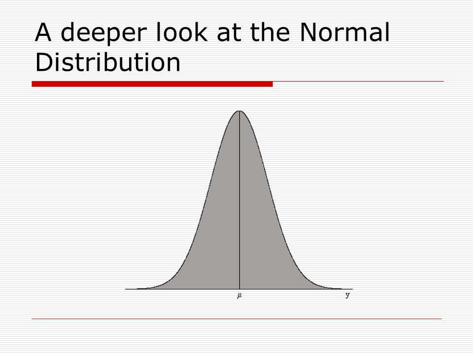
44. Poincaré: “…everyone believes in the [Normal] law of errors, the experimenters because they think it is a mathematical theorem, the mathematicians because they think is an empirical fact.” A deeper look at the Normal Distribution

46.  The 68-95-99.7% Rule--all normal density curves satisfy the following property: 68% of the observations fall within 1 standard deviation of the mean 95% of the observations fall within 2 standard deviations of the mean 99.7% of the observations fall within 3 standard deviations of the mean A deeper look at the Normal Distribution

47. Useful Distributions  The  2 distribution The sum of independent standard normal r.v.s  The t distribution The ratio of a standard normal r.v. to the square root of an independent  2 r.v. divided by its d.o.f. (example in class, pg 93)  The F distribution The ratio of two  2 r.v.s divided by their respective d.o.f.

48.   And we can make probability statements about What is gained by assuming normally distributed errors?

49. Hypothesis testing  The purpose of a hypothesis test is to determine whether an estimation result is consistent with the theory that gave rise to the econometric model

50. Hypothesis testing  t -tests Significance of individual coefficient The equality of two individual coefficients A single linear restriction  Why are we using a t-test? ???  Recall that

51. Hypothesis testing  Then we have:

52.  The null hypothesis (H 0 ) and the alternative hypothesis (H 1 or H a )  Choose a significance level Typically the.05 (5%) level or the.01 (1%) level is used  Calculate a test statistic (e.g., t test ) Hypothesis testing

53.  Find the critical value of the test statistic (e.g., t critical derived from tables in the book)  Apply the following decision rule: If |test value| > critical value, then reject H o e.g., if |t test | > t critical, then reject H o if |t test | < t critical, then fail to reject H o WHY? ???? Hypothesis testing

54.  Economic theory suggests that domestic currency depreciation leads to higher inflation rates: Tradable goods effect Pass-through effect Hypothesis testing

55.  Lets test this theory. We will do this example in class!! Hypothesis testing

56.  Null hypothesis: ????  Alterative Hypothesis: ???? Hypothesis testing

57.  Select a significance level ???? Hypothesis testing 90% Significance99% Significance

58.  Sampling Distribution under Ho  Rejection Region Fail to Reject Region  Rejection Region Hypothesized Value Critical Values Hypothesis testing

59.  Calculate the test statistic: ??? Hypothesis testing

60.  Find the critical value: Note: the critical value depends on the significance level (for a two-tailed test, the significance level α is divided between the two tails) and the degrees of freedom (number of observations minus number of slope parameters to be estimated) Hypothesis testing

61.  Apply decision rule—  reject the null hypothesis? ??? Hypothesis testing

62. Hypothesis Testing  When doing hypothesis testing we have to keep in mind the possible errors that we can make: Type I Error  Rejecting a true null ??? Type II Error  Failing to reject a false null ???

63.  The probability value (p-value) of a statistical hypothesis test is the probability of getting a value of the test statistic as extreme as or more extreme than that observed by chance alone, if the null hypothesis H 0, is true.  The p-value is largest significance level resulting in acceptance of H 0.  It is the probability of wrongly rejecting the null hypothesis if it is in fact true. Hypothesis Testing

64.  It is equal to the significance level of the test for which we would only just reject the null hypothesis. The p-value is compared with the actual significance level of our test and, if it is smaller, the result is significant. That is, if the null hypothesis were to be rejected at the 5% significance level, this would be reported as "p < 0.05".  Small p-values suggest that the null hypothesis is unlikely to be true. The smaller it is, the more convincing is the rejection of the null hypothesis. It indicates the strength of evidence for say, rejecting the null hypothesis H 0, rather than simply concluding “Reject H 0 ” or “Fail to reject H 0 ” Hypothesis Testing

65.  Discussion about one-tailed tests ???  A note on How to choose the null hypothesis ??? Hypothesis Testing

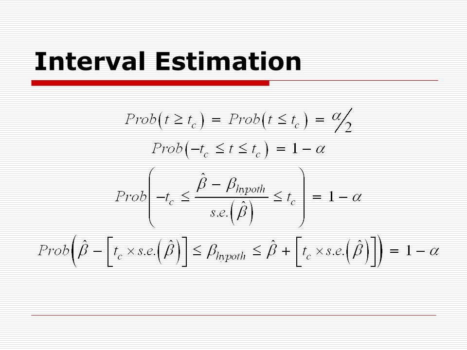
66.  Gives an estimated range of values which is likely to include an unknown population parameter, the estimated range being calculated from a given set of sample data. Note: it is another use of the t-statistic Interval Estimation

67.  The confidence level is the probability value (1 - ) associated with a confidence interval.  It is often expressed as a percentage. For example, say  = 0.05, or 5%, then confidence level = (1 - 0.05) = 0.95, that is, a 95% confidence level.  Why is this so? ??? Interval Estimation

69.  Interpretation anyone? ???  The width of the confidence.  Does it matter? ???  Point vs. interval estimator ??? Interval Estimation

70.  One of the objectives of the linear regression analysis is to predict the values of the dependent variable.  How can we make a prediction. ???  Do we have confidence interval for our predictions ???? (hint: think of another use of the t-statistic) Interval Estimation

71. The Simple Linear Regression Model: the R 2  After we have estimated the linear regression model we would like to be able to make statements about how much of the variation of the dependent variable is explained by the model.  In other words we want a measure of the proportion of variation in y explained by x within the regression model.

72. The Simple Linear Regression Model: the R 2  Recall that the SLRM has two components Non Random Random/stochastic

73. The Simple Linear Regression Model: the R 2  Graphically this means:

74. The Simple Linear Regression Model: the R 2  Then we have:

75. The Simple Linear Regression Model: the R 2  All we are looking for is a proportion measure.  With these sums we can get a ratio of the SSR and the SST. This ratio is called the R 2 or the coefficient of determination.

76. The Simple Linear Regression Model: the R 2  Interpretation of the R 2. ???

77. Final notes for the SLRM  Scaling the data  The SLRM is more powerful and useful than you think:  Choosing the Functional Form  The usefulness of the Normal Distribution shows up again!!