1. Generating Streams with Torus Models Paul McMillan Lund/Oxford Ringberg Streams meeting, July 2015 Collaborators: James Binney, Jason Sanders

2. Modelling streams (not orbits) Streams don’t follow orbits. Streams exist because stars are put onto different orbits. Streams show us the difference between orbits

3. Obligatory “what are angles, frequencies & actions” slide There is no way this hasn’t already been explained at this meeting. Orbits have conserved action J, with conjugate angle θ, which increases linearly with frequency Ω(J) Not simple to determine these.

4. Obligatory “what are angles, frequencies & actions” slide There is no way this hasn’t already been explained at this meeting. Orbits have conserved action J, with conjugate angle θ, which increases linearly with frequency Ω(J) Not simple to determine these.

5. Basics of stream formation in action angle coordinates Stars stripped from a satellite progenitor (typically) have a small spread in J about that of the progenitor (J p ) & and a value of θ close to that of the progenitor (at the time it was stripped). The stars move away from the satellite because they have a different orbital frequency Ω(J) ≠ Ω(J p ) One of the three eigenvalues of D is much larger than the other two (Helmi & White 1999, Eyre & Binney 2011)

6. Finding the Galactic potential with a stream Sanders (2104) shows that one can determine the potential of a Galaxy by fitting a frequency-angle stream model to a stream. But even with wildly optimistically small errors, finding a likelihood takes ages, because integrating over errors requires very fine resolution in high dimensions.

7. Schematically v1 v2 Observational uncertainty Model So the integral takes ages because one has to cover the whole area but then focus on relevant area of unknown shape/size The problem with working in x,v:

8. Stream modelling with tori: Methodology Torus modelling takes a fixed potential, a value J, and determines (by a fitting process) all of the corresponding orbit (the orbital torus). Provides an analytic expression for (x,v)(θ) for that J Quick to find the values of v & θ corresponding to a given x (if the orbit crosses that point) As yet, implemented for axisymmetric potentials only (https://github.com/PaulMcMillan-Astro/Torus) It works by manipulating the relationship between J,θ & x,v in a ‘toy’ potential to one that applies in the potential you care about… McGill & Binney 1990, Kaasalainen & Binney (1994a,1994b), McMillan & Binney (2008)

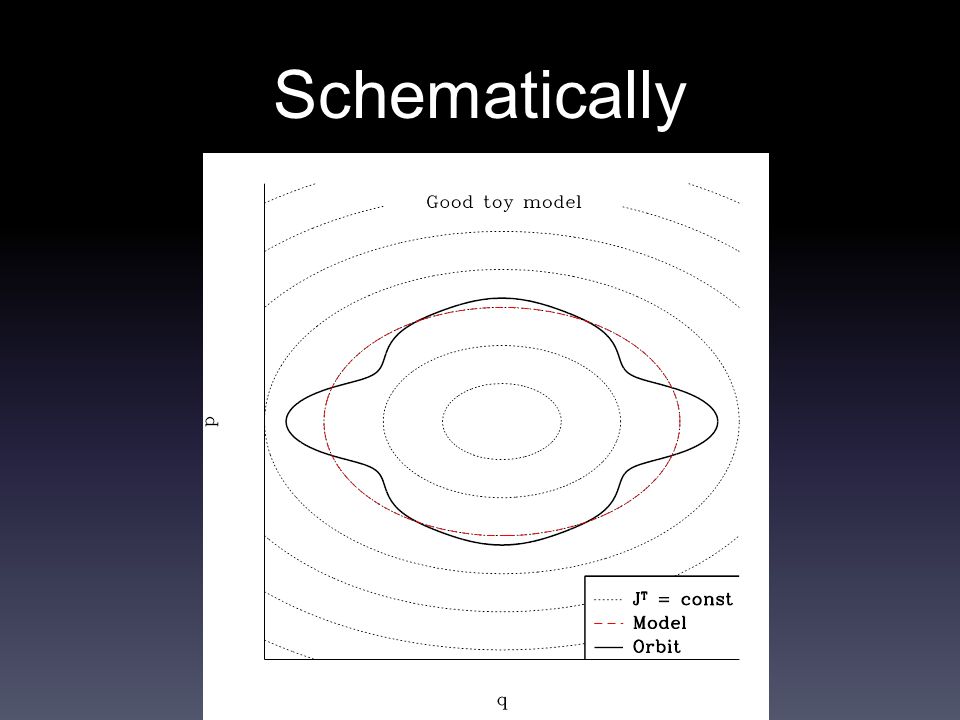
9. Stream modelling with tori: Methodology We know (J,θ)  (x,v) analytically for orbits in the effective, generalised isochrone potential McGill & Binney 1990, Kaasalainen & Binney (1994a,1994b), McMillan & Binney (2008) We refer to the values found here (for a given x, v and isochrone parameters) as J T and θ T. To find a torus with actions J in a Galactic potential Φ, we just need to retain key properties of the surface J T = const, while ensuring that the surface J=const is at const energy.

10. Stream modelling with tori: Methodology McGill & Binney 1990, Kaasalainen & Binney (1994a,1994b), McMillan & Binney (2008) Free to choose parameters of the toy potential: We then use a ‘generating function’ designed to find the required variation of J T as a function of θ T for a given value of J. Parameters are chosen to minimise variation of the Hamiltonian over a set of points equally spaced in θ T over the torus. Each ‘fit’ takes ~ 0.05s.

11. Schematically

15. Multiple Tori

16. Interpolation between tori First used by Kaasalainen (1994) in the construction of tori for resonant orbit families. Here simply used to allow rapid conversion between J,θ and x,v in the regime of interest. There can be a complicated interplay between parameters of toy potential & the values S n. Assign (smoothly varying) values for toy potential parameters, and set Sn free. Interpolate Sn (and param of toy) linearly in J in 3D grid…

17. Interpolation - example Take a grid with corners at J R = 0.4,0.6; J z =0.4,0.6; J ϕ =3.2,3.9 (code units – multiply by ≈1000 for kpc km/s) Fit 8 tori (each corner) First check- energy conservation. Set sensible threshold for fit of the 8 tori (σ H ≈ 0.001 * max K.E.) Interpolated tori (almost) fit same condition (typical σ H ≈ 0.0011 * max K.E.). But do they follow orbits?

18. Interpolation - example Tori interpolated in this grid clearly still correspond (pretty closely) to orbits Any small ‘drift’ is systematic in J (not random)

19. Interpolation - example Tori interpolated in this grid clearly still correspond (pretty closely) to orbits Any small ‘drift’ is systematic in J (not random)

20. Populate stream models We have a simple route to (quickly) go from J,θ to x,v in a range of J (Streams are typically very clumped in J) It is now trivial to populate a model described in J, θ. Simplest example - Gaussian blob in J, Δθ = ΔΩ(J)t BUT we know that there is a gap in the Ω(J) plane: Sanders (2014) Bovy (2014)

21. So, Gaussians in Ω,θ? There’s a near linear relationship between Ω & J Gaussian Ω  Gaussian J, but: Eyre & Binney 2011 Bovy 2014 Fardal et al.201 5 J space shows the structure much more clearly

22. A Simple model Combine insights that we have gap in one component of Ω, and bowtie structure in J. Pick a direction in J (e.g. corresponding to largest eigenvalue of δΩ/δJ, but YMMV). Call this J ||. We have an approximate idea for the the spread in each component of J & θ (following Eyre & Binney 2011 & Bovy 2014) Take projection of σ in J ||, to give dispersion in leading & trailing tails. Each is displaced in J λ by ~ 5-6 σ || from progenitor (Sanders 2014, Bovy 2014). and

23. Bowtie structure Simple way to get the bowtie structure – set dispersion perpendicular to J || an increasing fn of δJ || e.g. ~ (1+tanh(δJ || /2σ || )) Release stars uniformly in time (to some t max ), let them move away from the progenitor.

24. We have a stream model ~ 0.5s to fit tori, sample ~ 20,000 J,θ values/s

25. But this doesn’t solve all problems… l b Model Observation The problem with working in J,θ:

26. Tantalizing possibility We have analytic expressions for x,v at a given J,θ for all θ in a range of J We therefore also have differentials of x,v w.r.t. J,θ – we should be able to quickly find J,θ for any x,v (within this range in J) We already do this to find v at given x for given (fixed) J This would 1)make finding likelihoods for models given obs. data far easier. 2)Allow use of more complicated models (e.g. Fardal et al 2014)

28. “Streams” after many dynamical times (McMillan & Binney 2008) After many dynamical times a disrupted satellite can appear well phase mixed. Even if it covers a relatively large volume of J space, a Ω-θ relation remains. Observe in limited θ range (e.g. locally) and the Ω (or J) distribution is clumped

29. Note – spacing in Ω gives estimate of disruption time, potential Use a simple statistic that is 0 if all stars would (following their progress back) be at the same angle a time t’ ago. Finds t’ if given the correct potential, and doesn’t reach a significant minimum if given a bad one. Clearly rather crude – what about more realistic cases?

30. Live disc & halo Gomez & Helmi (2010) looked at the question of whether you could determine the accretion time for a (massive) satellite in a responsive disc galaxy. Still clumpy in frequency No direct use of the angles (rely on small volume) Take power spectrum of Fourier transform of frequency space. Still find a peak at the spacing one would expect for true time of disruption.

32. Conclusions Torus modelling provides a convenient way of quickly generating stream models, working in the model coordinates. Interpolation between tori means we don’t have to go through a whole faff for each new value J in a stream model We can (soon?) go in both directions between J, θ and x,v in a range of J Is it possible to use advances in action-angle methods to go further than previously with well mixed streams?