1. Search 3

2. Uniform-Cost Search
When all step costs are equal, breadth-first search is optimal because it always expands the shallowest unexpanded node.
By a simple extension, we can find an algorithm that is optimal with any step-cost function.
Instead of expanding the shallowest node, uniform-cost search expands the node n with the lowest path cost g(n).
This is done by storing the frontier as a priority queue ordered by g.

3. Uniform-Cost Search
Same idea as the algorithm for breadth-first search…but…
Expand the least-cost unexpanded node (whereas BFS expands the shallowest unexpanded node)
FIFO queue is ordered by cost
Equivalent to regular breadth-first search if all step costs are equal

4. Uniform-Cost Search vs. BFS
1) Ordering of the queue by path cost
2) The goal test is applied to a node when it is selected for expansion (same as the generic graph-search algorithm) rather than when it is first generated.
The reason is that the first goal node that is generated may be on a suboptimal path.
3) A test is added in case a better path is found to a node currently on the frontier.

5. General Graph search algorithm

6. Uniform-Cost Search (UCS)
Uniform-cost search on a graph
UCS algorithm is identical to the general graph search algorithm with following differences
A priority queue for frontier and the
Addition of an extra check in case a shorter path to a frontier state is discovered.
The data structure for frontier needs to support efficient membership testing
so it should combine the capabilities of a priority queue and a hash table.

7. Uniform-Cost Search
function UNIFORM-COST-SEARCH(problem) returns a solution, or failure
Node.STATE = problem.INITIAL-STATE, PATH-COST = 0
frontier <- a priority queue ordered by PATH-COST, with node as the only element
explored <- an empty set
loop do
if EMPTY?(frontier) then return failure
node <- POP(frontier) /* chooses the lowest-cost node in frontier */
if problem.GOAL-TEST(node.STATE) then return SOLUTION( node)
add node.STATE to explored
for each action in problem.ACTIONS(node.STATE) do
child <- CHILD-NODE(problem, node, action)
if child.STATE is not in explored or frontier then
frontier <- INSERT( child ,frontier)
else if child. STATE is in frontier with higher PATH-COST then
replace that frontier node with child

8. How to compute the components of a child node?
Given the components for a parent node, it is easy to see how to compute the necessary components for a child node.
The function CHILD-NODE takes a parent node and an action and returns the resulting child node

9. Romania with step costs in km
Uniform-cost search
Romania with step costs in km

10. Ex1: Uniform-Cost Search
Using UCS, find a path from Sibiu to Bucharest

11. Ex2: Uniform-cost search
Romania with step costs in km

12. Uniform-cost search Implementation:
frontier = queue ordered by path cost
So, the queue keeps the node list sorted by increasing path cost
Expands the first unexpanded node (hence with smallest path cost)
Does not consider the number of steps a path has, but only on their total cost
The Uniform cost search finds the cheapest solution provided a simple requirement is met: ie., the cost of a path must never decrease as we go along the path.

13. Uniform-Cost Search Optimal
Yes, Nodes are expanded in increasing order of path cost
So, cost of a path always increases as we go along the path
So, the first goal node selected for expansion is the optimal solution
1) whenever uniform-cost search selects a node n for expansion, the optimal path to that node has been found.
2) Because step costs are nonnegative, paths never get shorter as nodes are added.
These two facts together imply that uniform-cost search expands nodes in order of their optimal path cost.
Hence, the first goal node selected for expansion must be the optimal solution.

14. Uniform-Cost Search Completeness:
Uniform-cost search does not care about the number of steps a path has, but only about their total cost.
Therefore, it will get stuck in an infinite loop if there is a path with an infinite sequence of zero-cost actions
Example: a sequence of NoOp actions.
Completeness is guaranteed provided the cost of every step exceeds some small positive constant E.
if the cost is greater than or equal to some small positive constant
step cost >= ε

15. Uniform Cost Search - Time Complexity
In the worst case
every edge has the minimum cost e.
c* is the cost of optimal solution, so once all nodes of cost  c* have been chosen for expansion, a goal must be chosen
The maximum length of any path searched up to this point cannot exceed c*/e, and hence the worst-case number of such nodes is bc*/e .
Thus, the worst case asymptotic time complexity of UCS is
O(bc*/e )

16. Uniform-Cost Search
Complexity analysis depends on path costs rather than depths
Time
Complexity cannot be determined easily by d or d
Let C* be the cost of the optimal solution
Assume that every action costs at least ε
O(b 1+ ceil(C*/ ε))
Space
O(b 1+ceil(C*/ ε))
Note: Uniform cost explores large trees of small steps
So, b1+ceil(C*/ ε) can be much greater than b d+1
If all step costs are equal then b1+ceil(C*/ ε) is equal to bd+1

17. UCS vs. BFS
When all step costs are the same, uniform-cost search is similar to breadth-first search except
BFS stops as soon as it generates a goal, whereas
uniform-cost search examines all the nodes at the goal's depth to see if one has a lower cost;
thus uniform-cost search does strictly more work by expanding nodes at depth d unnecessarily.

18. Uniform-cost search S B G C A 1 10 5 15

19. Uniform-cost search S B G C A 1 10 5 15
BFS will find the path SAG, with a cost of 11, but SBG is cheaper with a cost of 10
Uniform Cost Search will find the cheaper solution (SBG).

20. Depth-First Search
Recall from Data Structures the basic algorithm for a depth-first search on a graph or tree
Expand the deepest unexpanded node
Unexplored successors are placed on a stack until fully explored
Implementation- recursive function

22. DFS
Depth-first search always expands the deepest node in the current frontier of the search tree.
The search proceeds immediately to the deepest level of the search tree where the nodes have no successors.
As those nodes are expanded, they are dropped from the frontier
so then the search "backs up" to the next deepest node that still has unexplored successors.

23. DFS
The depth-first search algorithm is an instance of the graph-search algorithm
depth-first search uses a LIFO queue.
An alternative to the GRAPH-SEARCH-style implementation
it is common to implement depth-first search with a recursive function that calls itself on each of its children in turn

24. DFS
The properties of depth-first search depend strongly on whether the graph-search or tree-search version is used.
The graph-search version avoids repeated states and redundant paths
is complete in finite state spaces because it will eventually expand every node.
The tree-search version is not complete
In Romania map, the algorithm will follow the Arad-Sibiu-Arad-Sibiu loop forever.

25. DFS Depth-first tree search can be modified at no extra memory cost
so that it checks new states against those on the path from the root to the current node;
this avoids infinite loops in finite state spaces but does not avoid the proliferation of redundant paths.
In infinite state spaces, both versions fail if an infinite non-goal path is encountered.

26. DFS For similar reasons, both versions are non optimal.
Ex: What happens if C is a goal node?
depth first search will explore the entire left subtree even if node C is a goal node.
Hence, depth-first search is not optimal.

28. DFS
The time complexity of depth-first graph search is bounded by the size of the state space (which may be infinite, of course).
A depth-first tree search, on the other hand, may generate all of the O(bm) nodes in the search tree, where m is the maximum depth of any node;
This can be much greater than the size of the state space.
Note that m itself can be much larger than d (the depth of the shallowest solution) and is infinite if the tree is unbounded.

29. Max depth m and depth of goal node db d m

30. General Graph search algorithm

31. Informal Description of search tree Algorithm

32. DFS
So far, depth-first search seems to have no clear advantage over breadth-first search, but there is space complexity
The reason is the space complexity.
For a graph search, there is no advantage
but a depth-first tree search needs to store only a single path from the root to a leaf node, along with the remaining unexpanded sibling nodes for each node on the path.
Once a node has been expanded, it can be removed from memory as soon as all its descendants have been fully explored.

33. DFS
For a state space with branching factor b and maximum depth m, depth-first search requires storage of only O(bm) nodes.
Using the same assumptions assuming that nodes at the same depth as the goal node have no successors
we find that depth-first search would require 156 kilobytes
instead of 10 exabytes at depth d = 16, a factor of 7 trillion times less space.
This has led to the adoption of depth-first tree search as the basic workhorse of many areas of AI
For the remainder of this section, we focus primarily on the tree search version of depth-first search.

34. Exponential Growth for BFS
1000 Bytes = 1 Kilobyte · 1000 Kilobytes = 1 Megabyte · 1000 Megabytes = 1 Gigabyte · 1000 Gigabytes = 1 Terabyte · 1000 Terabytes = 1 Petabyte · 1000 Petabytes = 1 Exabyte

35. Exponential Growth for DFS
Repeat the previous table for DFS

36. Depth-first search: Observations
If DFS goes down a infinite branch it will not terminate if it does not find a goal state.
If it does find a solution there may be a better solution at a lower level in the tree. Therefore, depth first search is neither complete nor optimal.

37. Depth-First Search Space
It needs to store only a single path from the root to a leaf node along with unexpanded sibling node for each node on the path
Once a node has been expanded, it can be removed from memory as soon as all its descedants are explored
For a state space with a branching factor of b and a maximum depth of m, DFS requires storage of bm + 1 nodes
O(bm)…linear space

38. Space complexity of depth-first
Largest number of nodes in QUEUE is reached in bottom left-most node.
Example: m = 3, b = 3 :
...
QUEUE contains all 10 nodes.
In General: (b * m) + 1
Space : O(m*b)

39. Time complexity of depth-first: details
In the worst case:
the (only) goal node may be on the right-most branch, m b G
Time complexity == bm + bm-1 + … + 1
Thus: O(bm)

40. Depth-First Search

41. Depth-First Search

42. Depth-First Search

43. Depth-First Search

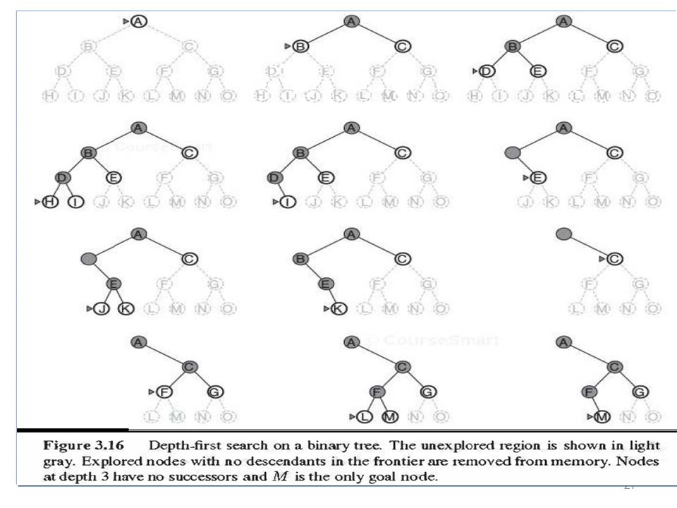
44. Depth-First Search
Black nodes – Nodes that are expanded and have no descendants in the frontier can be removed from memory

45. Depth-First Search

46. Depth-First Search

47. Depth-First Search

48. Depth-First Search

49. Depth-First Search

50. Depth-First Search

51. Depth-First Search
Assume M is the only goal node

52. Depth-first search B C E D F G S A

53. PROBLEM: Depth-first search
Run Depth First Search on the search space given above, and trace its progress.

54. Romania with step costs in km
Depth-first search
Romania with step costs in km

55. Depth-first search

56. Depth-first search

57. Depth-first search

58. Variant of DFS Backtracking search uses still less memory.
In backtracking, only one successor is generated at a time rather than all successors;
each partially expanded node remembers which successor to generate next.
In this way, only O(m) memory is needed rather than O(bm).

59. Variant of DFS
Backtracking search with another memory-saving and time-saving trick:
the idea of generating a successor by modifying the current state description directly rather than copying it first.
This reduces the memory requirements to just one state description and O(m) actions.
For this to work, we must be able to undo each modification when we go back to generate the next successor.
Note: For problems with large state descriptions, such as robotic assembly, these techniques are critical to success.

60. Depth-limited search (DLS) vs DFS
DFS may never terminate as it could follow a path that has no solution on it
DLS solves this by imposing a depth limit, at which point the search terminates at that particular branch
DLS = depth-first search with depth limit l ,

61. Depth-Limited Search
A variation of depth-first search that uses a depth limit
Alleviates the problem of unbounded trees
Search to a predetermined depth l (“ell”)
Nodes at depth l are treated as if they have no successors
Same as depth-first search if l = ∞
Two types of failure: Can terminate for failure (no solution) and cutoff (no solution within the depth limit l

62. Depth-limited search: Observations
Choice of depth parameter is important
Too deep is wasteful of time and space
Too shallow and we may never reach a goal state

63. Depth limits can be based on the knowledge of the problem
Bucharest
Zerind
Arad
Timisoara
Lugoj
Mehadia
Dobreta
Craiova
Rimnicu Vilcea
Sibiu
Pitesti
Giurgui
Urziceni
Hirsova
Eforie
Vaslui
Iasi
Neamt
Odarea
Fararas
On the Romania map there are 20 towns so any town is reachable in 19 steps
So, if there is a solution, it must be of length 19 at the longest
So set (l =19)
What is the max number of steps to reach from any city to any other city

64. Depth limits can be based on the knowledge of the problem
This number known as diameter of the state space
Gives a better depth limit
DLS can be used when there is a prior knowledge to the problem, which is always not the case
Typically, we will not know the depth of the shallowest goal of a problem unless we solved this problem before.

65. Depth-limited search Optimality
Completeness
If we choose l < d then it is incomplete
Therefore it is complete if l >=d (d=depth of solution)
If the depth parameter, l , is set deep enough then we are guaranteed to find a solution if one exists
Complete: if l is chosen appropriately then it is guaranteed to find a solution.
Optimality
DLS is not optimal if we choose l > d
Not Optimal: As it does not guarantee to find the least-cost solution
Space requirements are O(bl )
Time requirements are O(bl )

66. Depth-Limited Search Complete Time Space Optimal Yes if l >= d
O(bl)
Space
Optimal
No if l > d

67. Depth-limited search Recursive implementation:
depth-limited search can terminate with two kinds of failure:
failure value indicates no solution;
cutoff value indicates no solution within the depth limit.

68. DEPTH LIMITED TREE SEARCH

69. Iterative Deepening Search
Iterative deepening depth-first search
Uses depth-first search
Finds the best depth limit for DFS
Gradually increases the depth limit; 0, 1, 2, … until a goal is found
This will occur when the depth limit reaches d, the depth of the shallowest goal node

70. Iterative Deepening Search
The iterative deepening search algorithm Returns a solution or failure
repeatedly applies depth limited search with increasing limits.
It terminates when a solution is found or if the depth limited search returns failure meaning that no solution exists .

71. Iterative deepening search
Procedure
Successive depth-first searches are conducted – each with depth bounds increasing by 1

72. Iterative deepening search
First do DFS to depth 0
(i.e., treat start node as having no successors),
then, if no solution found,
do DFS to depth 1, etc.

73. Iterative Deepening Search

74. Iterative Deepening Search

75. Iterative Deepening Search

76. Iterative Deepening Search
Note: Solution is found at 4th iteration

77. Iterative Deepening Search
In practice, however, the overhead of these multiple expansions is small, because most of the nodes are towards leaves (bottom) of the search tree:
the nodes that are evaluated several times(towards top of tree) are in relatively small number.
In iterative deepening, nodes at bottom level are expanded once, level above twice, etc. up to root (expanded d+1 times)

78. Iterative deepening search
Number of nodes generated in a breadth-first search to depth d with branching factor b:
NBFS = b + b2 + … + bd
Number of nodes generated in an iterative deepening search to depth d with branching factor b:
NIDS = (d+1)b0 + d b1 + (d-1)b2 + … + (1)bd = O(bd)
For b = 10, d = 5,
NBFS = , , ,000 = 1,11, 111
NIDS = , , ,000 = 1,23,456
Note: There is some extra cost for generating the upper levels multiple times, but it is not large in IDS.

79. Lessons From Iterative Deepening Search
IDS may seem wasteful as it is expanding the same nodes many times.
A hybrid approach with BFS and IDS
run breadth-first search until almost all the available memory (frontier) is consumed, and then
runs iterative deepening from all the nodes in the frontier.
In general, iterative deepening search is the preferred uninformed search method when there is a large search space and the depth of the solution is not known

80. Iterative Deepening Search
IDS combines the benefit of DFS and BFS
IDS inherits BFS property
IDS explores a complete layer of new nodes at each iteration before going on to the next layer
BFS benefits
Completeness is ensured if b is finite
Optimality is ensured when the path cost is a non decreasing function of the depth of the node
DFS benefits
Space : O(bd)

81. Iterative deepening search: observations
Time Complexity = O(bd)
Space Complexity = O(bd)

82. Properties of iterative deepening search
Complete? Yes
Time? (d+1)b0 + d b1 + (d-1)b2 + … + bd = O(bd)
Space? O(bd)
Optimal? Yes, if step cost = 1

83. BDS

84. Bi-directional search (BDS)
Simultaneously two searches:
Search forward from initial state
Search backward from the goal
Stop when the two searches meet in the middle.

85. Bi-directional search
Goal
Start

86. Bi-directional search
Bidirectional search is implemented by
replacing the goal test with a check to see whether the frontiers of the two searches intersect;
if they do, a solution has been found.
Optimality:
It is important to realize that the first such solution found may not be optimal, even if the two searches are both breadth-first;
some additional check is required.
The check can be done when each node is generated or selected for expansion
With a hash table, such check will take constant time.

87. Bi-directional search
Much more efficient.
If branching factor = b in each direction, with solution at depth d
Rather than doing one search of bd, we do two bd/2 searches.
bd/2 + bd/2 is much less than bd
Example:
• Suppose b = 10, d = 6. Suppose each direction runs BFS
• In the worst case, two searches meet when each search has generated all of the nodes at depth 3.
Breadth first search will examine 11, 11, 111 nodes.
• Bidirectional search will examine 2,220 nodes.

88. Bi-directional search
Time complexity: 2*O(bd/2) =O(bd/2)
Space complexity: O(bd/2)
Example Contd …
• For the same b = 10, d = 6. What is the space complexity if one of the search is done by IDS ?
We can reduce the space complexity by roughly half if one of the two searches is done by iterative deepening,
But at least one of the frontiers must be kept in memory so that the intersection check can be done.
This space requirement is the most significant weakness of bidirectional search.

89. Bi-directional search

90. Bi-directional search - Implementation
for bidirectional search to work well, there must be an efficient way to check whether a given node belongs to the other search tree.
Either one or both searches should check each node before it is expanded to see if it is in the frontier of the other search tree
If so, a solution has been found

91. Bi-directional search
1.FRONTIER1 <- path only containing the root; FRONTIER2 <- path only containing the goal; 2. WHILE both FRONTIERs are not empty AND FRONTIER1 and FRONTIER2 do NOT share a state DO remove their first paths; create their new paths (to all children); reject their new paths with loops; add their new paths to back; 3. IF FRONTIER1 and FRONTIER2 share a state THEN success; ELSE failure;

92. Bi-directional search
Checking a node for membership in the other search tree can be done in constant time with a hash table
So, the time complexity of bidirectional search is O(bd/2)
Strength of BDS: time complexity
Atleast one of the search tree must be kept in memory so that the membership check can be done
So, the space complexity of bidirectional search is O(bd/2)
Limitation of BDS: space requirement (in comparison to DFS)
What is the best search strategy for the bidirectional searches?
It is complete and optimal if both searches are BFS
Other combinations may sacrifice completeness or optimality

93. Bi-directional search
Completeness: Yes,
Time complexity: 2*O(bd/2) =O(bd/2)
Space complexity: O(bd/2)
Optimality: Yes
To avoid one by one comparison, we need a hash table of size O(bd/2)
If hash table is used, the cost of comparison is O(1)

94. Bi-directional search
How do we search backwards from goal?
One should be able to generate predecessor states.
Predecessors of node x are all the nodes that have x as successor.
When all the actions in the state space are reversible, the predecessors of x are just its successors.
Suppose that the search problem is such that the arcs are bidirectional. That is, if there is an operator that maps from state A to state B, there is another operator that maps from state B to state A.
Other cases may require substantial ingenuity.

95. Bi-directional search
Problem: How do we search backwards from goal??
For goal states, apply predecessor function to them just as we applied successor function in forward search
Predecessor of a node n, Pred(n) = all those nodes that have n as a successor
1) BDS requires that Pred(n) be efficiently computable
Easy only when actions in the state space are reversible
This may not be the case always

96. Bi-directional search
Problem: How do we search backwards from goal??
2) Works well only if goals are explicitly known;
If there are several explicitly listed goal states, (ex: two dirt free states in vacuum problem)
Construct a new dummy goal state whose immediate predecessors are all the actual goal states
//redundant node generation

97. Bi-directional search
Problem: How do we search backwards from goal??
3) Difficult if goals are only characterized implicitly for a possibly large set of goals
Example: in Chess ?
lots of states satisfy that goal of check mate
no general way to do efficiently
A backward search should construct state descriptions “leading to check mate by move m” and then it should be tested against the states generated by forward search

98. Summary of algorithms This comparison is for tree-search versions.
For graph searches:
depth-first search is complete for finite state spaces and that the space and time complexities are bounded by the size of the state space.
b = Maximum branching factor of the search tree
d = Depth of least-cost solution
m = Maximum depth of the search tree (may be infinity)
l = Depth Limit or cut-off

99. Summary of algorithms YES a YES a,b NO YES a,d O(bd) O(b1+ C*/e) O(bm)
Criterion
Breadth-First
Uniform-cost
Depth-First
Depth-limited
Iterative deepening
Bidirectional search
Complete?
YES a
YES a,b NO
YES a,d
Time
O(bd)
O(b1+ C*/e)
O(bm) bl
O(bd/2)
Space
Optimal?
YES c
YES
YES c,d
a complete if b is finite
b complete if step cost >= e for positive e
c optimal if all step costs are identical
d if both directions use BFS