1. Sorting Lower Bounds n Beating Them

2. Recap Divide and Conquer –Know how to break a problem into smaller problems, such that –Given a solution to the smaller problems we can easily find a solution to the bigger problem

3. Recap Divide and Conquer –Divide and solve the smaller pieces recursively –Solve the big problem using the solutions to the smaller problems.

4. Recap The Quicksort algorithm: –chooses an element, called pivot. –Splits the input into three groups: smaller than the pivot equal to pivot larger than pivot. – Recursively sort the smaller and the larger groups independently

5. Quicksort Quicksort is one of the fastest algorithms known for sorting. For optimum efficiency, the pivot must be chosen carefully “Median of three” is a good technique for choosing the pivot

6. QuickSelect How do we modify randomized quicksort to find the k-th largest number in a given array? (Median finding?) Just recurse on one subarray, S L or S G or S = Picking a random pivot keeps the expected running time bounded. What is the expected running time?

7. Quickselect The expected height of the tree is still O(log n). But not the algorithm traces a path in the tree. T(n) <= T(3n/4) + O(n) for good pivots. Note that there is no 2 as was the case in quicksort. What does this recurrence solve to?

8. How fast can we sort? Can we do better than O(n lg n)? Well… it depends? It depends on the model of computation!

9. Comparison sorting Only comparisons are used to determine the order of elements Example –Selection Sort –Insertion sort –Merge Sort –Quick Sort –Heapsort

10. Lower Bounds How do we prove that any algorithm will need cnlogn time in the worst case? First Assumption: All these algorithms are allowed to only compare elements in the input. (Say only < ?)

11. I choose a permutation of {1,2,3,…N} Comparison Sort Game I ask you yes/no questions. Time is the number of questions asked in the worst case. I answer. I determine the permuation.

12. Decision Trees Another way of looking at the game Example: 3 element sort (a 1, a 2, a 3 ) One yes/no question? (Is x < y?) a 1 ? a 2 “Less than” leads to left branch “Greater than” leads to right branch

13. Decision Trees Example: 3 element sort (a 1, a 2, a 3 ) a 1 ? a 2 a 2 ? a 3

14. Decision Trees Example: 3 element sort (a 1, a 2, a 3 ) a 2 ? a3a 1 ? a 2 a 1, a 2, a 3

15. Decision Trees Example: 3 element sort (a 1, a 2, a 3 ) a 2 ? a 3 a 1 ? a 2 a 1 ? a 3 a 2 ? a 3 a 1 ? a 3 a 1, a 2, a 3 a 3, a 1, a 2 a 1, a 3, a 2 a 2, a 1, a 3 a 2, a 3, a 1 a 3, a 2, a 1

16. Decision Trees Each leaf contains a permutation indicating that permutation of order has been established A decision tree can model a comparison sort

17. Decision Trees It is the tree of all possible instruction traces Running time = length of path Worst case running time = length of the longest path (height of the tree)

18. Bounding log N! N! = 1 × 2 × 3 × … × N / 2 × … × N N factors each at most N. N / 2 factors each at least N / 2.  N N N / 2  N/2N/2 N / 2 log( N / 2 )  log(N!)  N log(N) =  (N log(N)).

19. Lower bound for comparison sorting Theorem: Any decision tree that sorts n elements has height  (n lg n) Proof: There are n! leaves A height h binary tree has no more than 2 h nodes and it should be able to resolve all n! permutations.

20. Optimal Comparison Sorting Algorithms Merge sort Quick sort Heapsort

21. Another D&C Application Matrix Multiplication What other D&C algorithms have we seen so far? D&C algorithms are also better for cache health in general. (Less cache misses because the base cases fit in the cache.)

22. Matrix Multiplication Algorithms: When multiplying two 2  2 matrices [A ij ] and [B ij ] The resulting matrix [C ij ] is computed by the equations C 11 = A 11 B 11 + A 12 B 21 C 12 = A 11 B 12 + A 12 B 22 C 21 = A 21 B 11 + A 22 B 21 C 22 = A 21 B 12 + A 22 B 22 When the size of the matrices are n  n, the amount of computation is O(n 3 ), because there are n 2 entries in the product matrix where each require O(n) time to compute.

23. Recap: Extra Credit HW Prob. (a+ib)(c+id) = (ac-bd)+i(bc+ad) 4 multiplications to 3.

24. Strassen’s fast matrix multiplication algorithm: Strassen’s divide-and-conquer algorithm (1969) uses a set of 7 algebraic equations to compute the product entries C ij : DefineM 1 = (A 12 – A 22 )(B 21 + B 22 ) M 2 = (A 11 + A 22 )(B 11 + B 22 ) M 3 = (A 11 – A 21 )(B 11 + B 12 ) M 4 = (A 11 + A 12 )B 22 M 5 = A 11 (B 12 – B 22 ) M 6 = A 22 (B 21 – B 11 ) M 7 = (A 21 + A 22 )B 11 One can verify by algebra that these M terms can be used to compute the C ij terms as follows: C 11 = M 1 + M 2 – M 4 + M 6 C 12 = M 4 + M 5 ; C 21 = M 6 + M 7 C 22 = M 2 – M 3 + M 5 – M 7

25. Strassen’s Algorithm When the dimension n of matrices is a power of 2, these equations can be used recursively in matrix multiplication. Thus, this algorithm’s computation time denoted T(n) satisfies the recurrence: Which solves to ? (Use master method?)

26. Radix Sort Based on Slides of L.F.Perrone Beating the lower bound for sorting

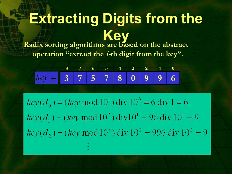
27. What is in a “Key” 375780996 Value in a base-R number system. We will call R the radix. R=10 (positional notation)

28. Extracting Digits from the Key Radix sorting algorithms are based on the abstract operation “extract the i-th digit from the key”. 375780996 876543210

29. Sorting on Partial Keys LSD Radix Sort 329 457 657 839 436 720 355 720 355 436 457 657 329 839 720 329 436 839 355 457 657 329 355 436 457 657 720 839 Look at the digits of the key one at a time starting from the least significant digit. For each i-th digit, sort the array using only that digit as the key for each array entry. Question: What property must the sorting algorithm have for this to work?

30. LSD Radix Sort Radix-Sort (A, d) for i=1 to d do stable sort array A on digit i Performance: Sorting N records with keys that have k digits requires k passes on the array. The total time for the sort will be k multiplied by the time for the sort on each digit of the key. Question: If you need to sort the array in linear time, what must be the run-time complexity of the stable sort you use?

31. Sorting in Linear Time Assumption: Each of the N elements in the array is an integer in the range 0 to k, for some integer k. 0 1 2 3 4 5 6 7 8 9 For some element i of the array, count how many other elements are smaller than i. This count indicates what position in the sorted array will contain i. If C[i]= 4, 4 elements in A are less than i. 0 1 2 3 4 5 6 7 8 9 i

32. Counting Sort Assumptions: –the input is in array A[1..n] and length(A)=n, –B[1..n] holds the sorted output, –C[0..k] holds count values (k=R-1)

33. Counting Sort Counting-Sort (A, B, k) for i=0 to k do C[i]=0 for j=1 to length(A) do C[A[j]] = C[A[j]]+1 for i=1 to k do C[i]=C[i]+C[i-1] for j=length(A) downto 1 do B[C[A[j]]]=A[j] C[A[j]]=C[A[j]]-1 C[i] contains the number of elements equal to i. C[i] contains the number of elements less than or equal to i. Questions: Is this stable? Is this in place? What is its run-time complexity?

34. Counting Sort Properties 1)The first loop takes time  (k). The second takes  (n). The third takes  (k). The fourth takes  (n). The overall time is  (n+k). If k=O(n), then counting sort takes time  (n)! 2)It is not a comparison sort. One can show that the lower bound for comparison sorts is  (n lg n). 3)It is stable. “Ties between two numbers are broken by the rule that whichever number appears first in the input array appears first in the output array.”

35. Counting Sort Example (R=6) 25302303 12345678 A 202301 012345 C 224778 012345 C 3 12345678 B 224678 012345 C 03 12345678 B 124678 012345 C 033 12345678 B 124578 012345 C

36. Hashing

37. Recall –Arrays : Unbeatable Property Have constant time access/update –Wish office[ “piyush” ] = 105B; meaning[ “serendipity” ] = “Good Luck in making unexpected and fortunate discoveries”; ssn[176902379].name = “John Galt”; Key

38. A String as a number “John” = 1,248,815,214 74 * 256^3 + 111 * 256^2 + 104 * 256^1 + 110

39. Hash Tables Hash table: –Given a table T and a record x, with key (= symbol) and satellite data, we need to support: Insert (T, x) Delete (T, x) Search(T, x) –We want these to be fast, but don’t care about sorting the records –In this discussion we consider all keys to be (possibly large) natural numbers

40. Direct Addressing Suppose: –The range of keys is 0..m-1 –Keys are distinct The idea: –Set up an array T[0..m-1] in which T[i] = xif x  T and key[x] = i T[i] = NULLotherwise –This is called a direct-address table Operations take O(1) time!

41. The Problem With Direct Addressing Direct addressing works well when the range m of keys is relatively small But what if the keys are 32-bit integers? (ssn) –Problem 1: direct-address table will have 2 32 entries, more than 4 billion –Problem 2: even if memory is not an issue, the time to initialize the elements to NULL may be Solution: map keys to smaller range 0..m-1 This mapping is called a hash function

42. Hash Functions Next problem: collision (pigeonhole) T 0 m - 1 h(k 1 ) h(k 4 ) h(k 2 ) = h(k 5 ) h(k 3 ) k4k4 k2k2 k3k3 k1k1 k5k5 U (universe of keys) K (actual keys)

43. Resolving Collisions How can we solve the problem of collisions? Solution 1: chaining Solution 2: open addressing

44. Open Addressing Basic idea (details in Section 12.4): –To insert: if slot is full, try another slot, …, until an open slot is found (probing) –To search, follow same sequence of probes as would be used when inserting the element If reach element with correct key, return it If reach a NULL pointer, element is not in table Good for fixed sets (adding but no deletion) –Example: spell checking Table needn’t be much bigger than n

45. Chaining Chaining puts elements that hash to the same slot in a linked list: —— T k4k4 k2k2 k3k3 k1k1 k5k5 U (universe of keys) K (actual keys) k6k6 k8k8 k7k7 k1k1 k4k4 —— k5k5 k2k2 k3k3 k8k8 k6k6 k7k7

46. Chaining How do we insert an element? —— T k4k4 k2k2 k3k3 k1k1 k5k5 U (universe of keys) K (actual keys) k6k6 k8k8 k7k7 k1k1 k4k4 —— k5k5 k2k2 k3k3 k8k8 k6k6 k7k7

47. T k4k4 k2k2 k3k3 k1k1 k5k5 U (universe of keys) K (actual keys) k6k6 k8k8 k7k7 k1k1 k4k4 —— k5k5 k2k2 k3k3 k8k8 k6k6 k7k7 How do we delete an element? –Do we need a doubly-linked list for efficient delete?

48. Chaining How do we search for a element with a given key? —— T k4k4 k2k2 k3k3 k1k1 k5k5 U (universe of keys) K (actual keys) k6k6 k8k8 k7k7 k1k1 k4k4 —— k5k5 k2k2 k3k3 k8k8 k6k6 k7k7

49. Analysis of Chaining Assume simple uniform hashing: each key in table is equally likely to be hashed to any slot Given n keys and m slots in the table: the load factor  = n/m = average # keys per slot What will be the average cost of an unsuccessful search for a key?

50. Analysis of Chaining Assume simple uniform hashing: each key in table is equally likely to be hashed to any slot Given n keys and m slots in the table, the load factor  = n/m = average # keys per slot What will be the average cost of an unsuccessful search for a key? A: O(1+  )

51. Analysis of Chaining Assume simple uniform hashing: each key in table is equally likely to be hashed to any slot Given n keys and m slots in the table, the load factor  = n/m = average # keys per slot What will be the average cost of an unsuccessful search for a key? A: O(1+  ) What will be the average cost of a successful search?

52. Analysis of Chaining Assume simple uniform hashing: each key in table is equally likely to be hashed to any slot Given n keys and m slots in the table, the load factor  = n/m = average # keys per slot What will be the average cost of an unsuccessful search for a key? A: O(1+  ) What will be the average cost of a successful search? A: O(1 +  /2) = O(1 +  )

53. Analysis of Chaining Continued So the cost of searching = O(1 +  ) If the number of keys n is proportional to the number of slots in the table, what is  ? A:  = O(1) –In other words, we can make the expected cost of searching constant if we make  constant

54. Choosing A Hash Function Clearly choosing the hash function well is crucial –What will a worst-case hash function do? –What will be the time to search in this case? What are desirable features of the hash function? –Should distribute keys uniformly into slots –Should not depend on patterns in the data

55. Hash Functions: The Division Method h(k) = k mod m –In words: hash k into a table with m slots using the slot given by the remainder of k divided by m What happens to elements with adjacent values of k? What happens if m is a power of 2 (say 2 P )? What if m is a power of 10? Upshot: pick table size m = prime number not too close to a power of 2 (or 10)

56. Hash Functions: The Multiplication Method For a constant A, 0 < A < 1: h(k) =  m (kA -  kA  )  What does this term represent?

57. Hash Functions: The Multiplication Method For a constant A, 0 < A < 1: h(k) =  m (kA -  kA  )  Choose m = 2 P Choose A not too close to 0 or 1 Knuth: Good choice for A = (  5 - 1)/2 Fractional part of kA

58. Hash Functions: Worst Case Scenario Scenario: –You are given an assignment to implement hashing –You will self-grade in pairs, testing and grading your partner’s implementation –In a blatant violation of the honor code, your partner: Analyzes your hash function Picks a sequence of “worst-case” keys, causing your implementation to take O(n) time to search What’s an honest CS student to do?

59. Hash Functions Universal Hashing As before, when attempting to foil an malicious adversary: randomize the algorithm Universal hashing: pick a hash function randomly in a way that is independent of the keys that are actually going to be stored –Guarantees good performance on average, no matter what keys adversary chooses

60. Universal Hashing Ideal World : Keys are uniformly distributed. –Not true for Real World Applications Goal: Hash Functions that produce less collisions. –Produce a random table index and don’t depend on the keys Idea: –Select a hash function at random From a “good” set of functions. Independent of the keys. –Use randomization to foil the adversary. Remember Randomized Quicksort?

61. Designing a Universal Class of Hash Functions Choose a prime number p large enough so that every possible key k is in the range 0 to p – 1 – Z p = {0, 1, …, p - 1} – Z p * = {1, …, p - 1}

62. Designing a Universal Class of Hash Functions Define the following hash function h a,b (k) = ((ak + b) mod p) mod m,  a  Z p * and b  Z p The family of all such hash functions is H p,m = {h a,b : a  Z p * and b  Z p } The class H p,m of hash functions is universal

63. An Example Universal Hash Functions Example p = 17, m = 6 h a,b (k) = ((ak + b) mod p) mod m h 3,4 (8) = ((3  8 + 4) mod 17) mod 6 = (28 mod 17) mod 6 = 11 mod 6 = 5

64. Advantages Universal hashing provides good results on average, independently of the keys to be stored Guarantees that no input will always elicit the worst-case behavior ( very very unlikely for high number of collisions to happen ) The algorithm behaves differently with each execution Poor performance occurs only when the random choice returns an inefficient hash function – this has small probability

65. Universal Hashing Property With universal hashing the chance of collision between distinct keys k and l is no more than the 1/m chance of collision if locations h(k) and h(l) were randomly and independently chosen from the set {0, 1, …, m – 1}

66. MidTerm Review What we should know by now? –What are algorithms? What is the RAM model? – Linear Search / Binary Search (Analysis) –Time and Space Complexity –Mathematical Induction and proving mathematical/algorithmic facts using induction

67. MidTerm Review Solving Recurrences –Guess and Verify –Recursion Trees –Master Method –Shift/Cancel –How to get a recurrence for calculating the running time of a program.

68. Midterm Review What we should know by now? –Asymptotic Complexity. Upper, Lower and Tight bounds. Big-O, Theta, Omega, o() and other notations for time and space complexity. –Manipulating notations, Properties. –How to analyze simple algorithms/programs and tell their time and space complexity. –Summing Arithmetic, Geometric Series and other simple series. Harmonic Series. –Manipulating log()

69. Midterm Review Sorting –Brute force –Heapsort –Randomized Quicksort –Insertion Sort –Merge Sort –Counting Sort –Radix Sort Their running times, analysis. Lower bounds for comparison based sorting. Randomized selection in linear time.

70. Midterm Review Strassen’s Matrix Multiplication algorithm and the simple iterative algorithm. Hashing –Direct Addressing –Open Addressing –Chaining –Hash functions (division + mult method) –Universal hashing

71. MidTerm To do well in the exam –Make sure you understand what the homework asked for. –Make sure you can solve those and similar problems yourself without any help. –Make sure you sleep well before exam, I will expect you to think in the exam.