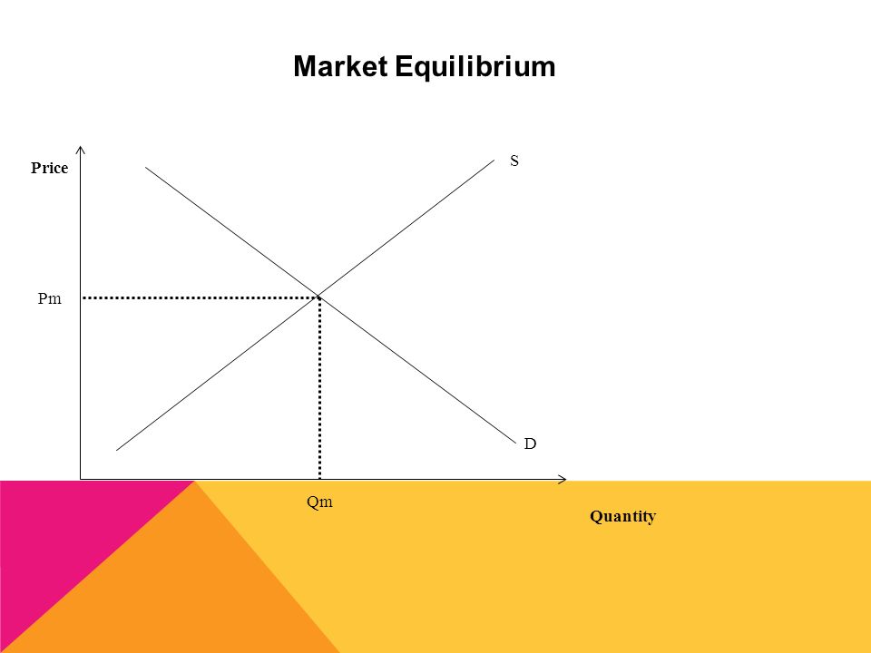
2. Market Equilibrium Price Quantity S D Pm Qm

3. At a Price Above Equilibrium Price Quantity S D Pm Qm P1 QsQd Qs > QD Surplus Too many goods and services Producers cut price Qd increases Qs decreases Return to equilibrium A surplus is where price is set above equilibrium causing QS>QD

4. At a Price Below Equilibrium Price Quantity S D Pm Qm P1 QdQs Qd > Qs Shortage Not enough goods and services Consumers bid up price Qd decreases Qs increases Return to equilibrium A shortage is where the price is set below equilibrium causing QD>QS

5. CONCLUSION A market will tend toward equilibrium If the price is not at equilibrium then market forces will work to move the market back toward equilibrium.

6. CONSUMER SURPLUS DEFINITION: MEASURED BY: The difference between what consumers are willing to pay and the actual price paid for a commodity

7. Consumer Surplus Price Quantity S D Pm Qm Consumer Surplus

8. Producer Surplus Definition: Measured by: The difference between the revenue received by a producer and the cost necessary to produce the good

9. Producer Surplus Price Quantity S D Pm Qm Producer Surplus

10. WHY IS EQUILIBRIUM BEST? Equilibrium represents the allocatively efficient point. This is where Consumer Surplus and Producer Surplus are maximised  ie benefits to consumers and producers are at their greatest Allocative Efficiency = A point where no one can be made better off without making someone worse off

11. WHICH IS THE ALLOCATIVELY EFFICIENT POINT? cars television A B 100 60 100 200

12. Which is the allocatively efficient point? cars television A B 100 60 100 200 quantity price Market for Cars S D 100

13. Which is the allocatively efficent point? cars television A B 100 60 100 200 quantity price Market for Cars S D 100

14. Net Welfare Benefit The combined values of the consumer and producer surpluses is referred to as the net welfare benefit. S D Pm Qm Net welfare benefit.

15. Allocative Efficiency and Market Equilibrium Markets allocate resources to the production of goods and services that satisfy consumers needs and wants. To be allocatively efficient a market must price and produce at equilibrium. Price Quantity S D 200 400 600 800 1.80 1.50 1.20 0.90 0.60 0.30 Any price other than $1.20 and any output level other than 400 units will result in a loss of allocative efficiency Resources would be either over or under allocated to production and net welfare benefit would be reduced. To maintain allocative efficiency a market must be able to move freely to any new equilibrium

17. Any changes in the market where the forces of demand and supply are able to freely adjust to market conditions will still result in allocative efficiency.

18. A loss of Allocative Efficiency A loss of allocative efficiency occurs when a market is not allowed to price and produce at equilibrium this will result from :  Price Controls(setting either a minimum or maximum price)  Imposition of a sales tax or subsidy  Imposition of a tariff or a quota (normally relates to internationally traded products) All of these regulations set by the government will result in a dead weight loss and thus causing net social welfare to fall.

19. DEADWEIGHT LOSS When a market does not achieve equilibrium producer and consumer surplus will not be maximised The loss in allocative efficiency is DWL It is measured by the loss of CS and PS not offset by gains to other groups (eg government)

20. Deadweight Loss Deadweight loss can be caused by: Quotas Price controls Indirect Taxes Subsidies

21. A Subsidy Price Quantity S D Pm Qm

22. A Subsidy Price Quantity S D Pm Qm Subsidies reduce costs and increase Supply S+Subsidy

23. A Subsidy Price Quantity S D Pm Qm Consumers pay the new equilibrium price - Pc S+Subsidy Q’ Pc

24. A Subsidy Price Quantity S D Pm Qm The per unit subsidy is represented by the vertical distance between the two supply curves S+Subsidy Q’ Pc

25. A Subsidy Price Quantity S D Pm Qm Producers receive higher price -Pp S+Subsidy Q’ Pc Pp

26. A Subsidy Price Quantity S D Pm Qm The total cost to the government is represented by the shaded area S+Subsidy Q’ Pc Pp

27. A Subsidy Price Quantity S D Pm Qm S+Subsidy Q’ Pc Pp Original CS

28. A Subsidy Price Quantity S D Pm Qm S+Subsidy Q’ Pc Pp New CS The gain in CS represents the incidence of a subsidy on consumers

29. A Subsidy Price Quantity S D Pm Qm S+Subsidy Q’ Pc Pp Old PS

30. A Subsidy Price Quantity S D Pm Qm S+Subsidy Q’ Pc Pp New PS The gain in PS represents the incidence of a subsidy on producers

31. A Subsidy Price Quantity S D Pm Qm S+Subsidy Q’ Pc Pp DWL

32. Before the Subsidy Price the consumers pay Price the producers receive Quantity sold Total spending by consumers Total revenue by producers Consumer surplus Producer surplus $ 2.50 100 000 $2.50 x 100 000 = 250 000

33. After the Subsidy Price the consumers pay Price the producers receive Amount of the subsidy = Quantity sold Total spending by consumers Total revenue by producers Consumer surplus Producer surplus Spending by Government Value of DWL $ 1.50 $ 1.50 +1.50 =$3.00 $ 1.50 200 000 1.50 x 200 000= 300 000 3.00 x 200 000= 600 000 1.50 x 200 000= 300 000

34. An Indirect Tax – Sales Tax Price Quantity S D Pm Qm

35. An Indirect Tax Price Quantity S D Pm Qm Indirect taxes increase costs and shift the supply curve to the left S+tax

36. An Indirect Tax Price Quantity S D Pm Qm Consumers pay the new equilibrium price - Pc S+tax Pc

37. An Indirect Tax Price Quantity S D Pm Qm The per unit tax is measured by the vertical distance between the two supply curves S+tax Q’ Pc

38. An Indirect Tax Price Quantity S D Pm Qm The producer recieves the lower price - Pp S+tax Q’ Pc Pp

39. An Indirect Tax Price Quantity S D Pm Qm The government receives the shaded area as tax revenue S+tax Q’ Pc Pp

40. An Indirect Tax Price Quantity S D Pm Qm S+tax Q’ Pc Pp Original CS

41. An Indirect Tax Price Quantity S D Pm Qm S+tax Q’ Pc Pp New CS The area of tax which was previously CS represents the incidence of the tax on consumers

42. An Indirect Tax Price Quantity S D Pm Qm S+tax Q’ Pc Pp Original PS

43. An Indirect Tax Price Quantity S D Pm Qm S+tax Q’ Pc Pp New PS The area of tax which was previously PS represents the incidence of the tax on producers

44. An Indirect Tax Price Quantity S D Pm Qm S+tax Q’ Pc Pp DWL

45. Before the tax Price the consumers pay Price the producers receive Quantity sold Total spending by consumers Total revenue by producers Consumer surplus Producer surplus Net Social Welfare = = $25 = 20 000 = 25 x 20 000 = $500 000 000s $250 000 + $ 200 000 $450 000

46. After the tax Price the consumers pay Price the producers receive Quantity sold Total spending by consumers Total revenue by producers Consumer surplus Producer surplus Revenue by Government Net Social Welfare Value of DWL = $30 = $30-10= $20 = 15 000 =30 x 15 000 = $450 000 = 20 x 15 000 = $ 300 000 = $10 x 15 000 = 150 000 $ 412500

47. Before the tax Price the consumers pay Price the producers receive Quantity sold Total spending by consumers Total revenue by producers Consumer surplus Producer surplus = $10 = 25 000 = 10 x 25000 = $250000 7 25

48. After the tax Price the consumers pay Price the producers receive Quantity sold Total spending by consumers Total revenue by producers Consumer surplus Producer surplus Revenue by Government Value of DWL = $15 = $15 -7= $8 = 20 000 = 15 x 20 000= 300000 = 8 x 20 000 = $160 000 Tax of $7 placed on RTDs $7 x 20 000= 140 000

49. Losses and Gains Before the tax CS = $312500 PS = $87500 Government Revenue = $0 DWL = $0 Total Gain to the economy = 400 000 Losses and Gains After the tax CS = $ 200000 ( Loss 112500) PS = $50 000 ( Loss 37500) Government Revenue = $140 000 Total Gain = $200000 + $50000 + 140 000 = $390 000

50. A Quota Price Quantity S D Pm Qm

51. A Quota Price Quantity S D Pm Qm In this example we assume there is no domestic production Q’

52. A Quota Price Quantity S D Pm Qm A quota is a limit on the number of imports into a country The supply curve becomes vertical at the quota level Q’

53. A Quota Price Quantity S’ D Pm Qm A quota is a limit on the number of imports into a country The supply curve becomes vertical at the quota level Q’ S

54. A Quota Price Quantity S’ D Pm Qm The new price is determined at the intersection of the new Supply curve and the original Demand curve - P’ Q’ S P’

55. A Quota Price Quantity S D Pm Qm Original CS Q’ P’

56. A Quota Price Quantity S D Pm Qm New CS Q’ P’

57. A Quota Price Quantity S D Pm Qm Old PS Q’ P’

58. A Quota Price Quantity S D Pm Qm New PS Q’ P’

59. A Quota Price Quantity S D Pm Qm DWL Q’ P’

60. A Maximum Price Price Quantity S D Pm Qm

61. A Maximum Price Price Quantity S D Pm Qm A maximum price is only effective when set below equilibrium price Pmax

62. A Maximum Price Price Quantity S D Pm Qm Qs decreases Although consumers would like to buy more producers only supply Qs There is a shortage Pmax Qs Qd

63. A Maximum Price Price Quantity S D Pm Qm Pmax Original CS Qs

64. A Maximum Price Price Quantity S D Pm Qm Pmax New CS Qs

65. A Maximum Price Price Quantity S D Pm Qm Pmax Original PS Qs

66. A Maximum Price Price Quantity S D Pm Qm Pmax New PS Qs

67. A Maximum Price Price Quantity S D Pm Qm DWL Pmax Qs

68. A Minimum Price Price Quantity S D Pm Qm

69. A Minimum Price Price Quantity S D Pmin Qm Pm A minimum price is only effective when set above equilibrium price

70. A Minimum Price Price Quantity S D Pmin Qm Pm Qd Qd decreases Although producers would like to sell more they are unable to at this high price

71. A Minimum Price Price Quantity S D Pmin Qm Pm Original CS Qd

72. A Minimum Price Price Quantity S D Pmin Qm Pm New CS Qd

73. A Minimum Price Price Quantity S D Pmin Qm Pm Original PS Qd

74. A Minimum Price Price Quantity S D Pmin Qm Pm New PS Qd

75. A Minimum Price Price Quantity S D Pmin Qm Pm DWL Qd

76. Net Welfare Benefit The combined values of the consumer and producer surpluses is referred to as the net welfare benefit. S D Pm Qm Net welfare benefit.

77. Allocative Efficiency and Market Equilibrium Markets allocate resources to the production of goods and services that satisfy consumers needs and wants. To be allocatively efficient a market must price and produce at equilibrium. Price Quantity S D 200 400 600 800 1.80 1.50 1.20 0.90 0.60 0.30 Any price other than $1.20 and any output level other than 400 units will result in a loss of allocative efficiency Resources would be either over or under allocated to production and net welfare benefit would be reduced. To maintain allocative efficiency a market must be able to move freely to any new equilibrium

78. Any changes in the market where the forces of demand and supply are able to freely adjust to market conditions will still result in allocative efficiency.

79. A loss of Allocative Efficiency A loss of allocative efficiency occurs when a market is not allowed to price and produce at equilibrium this will result from :  Price Controls(setting either a minimum or maximum price)  Imposition of a sales tax or subsidy  Imposition of a tariff or a quota (normally relates to internationally traded products) All of these regulations set by the government will result in a dead weight loss and thus causing net social welfare to fall.