1. EPI 5344: Survival Analysis in Epidemiology Week 6 Dr. N. Birkett, School of Epidemiology, Public Health & Preventive Medicine, University of Ottawa 03/2016 1 9. Left Truncation

2. Let’s start with a boring definition Subject being ‘under observation’ at time ‘t’ means: If subject had an event at time ‘t’, then subject would have been recorded with an event in the study. 03/2016 2

3. What is left truncation? A selection process which affects subjects so that their event time can not be lower than some time. Can occur in two ways Subject has event between time of eligibility and entry into observation Generally ‘unknown’ to cohort Subject has period of time from eligibility to start of observation when they have to be event free since they were selected at start of observation period 03/2016 3

4. What is left truncation? Subjects enter study at time ‘t 0 ’ During the time interval t 0  t 1, subject is not under observation Any event during this interval is missed Time of event for this subject is truncated Can not be earlier than t 1 03/2016 4

5. In fact, you often know nothing about the subject If the event is ’death’, they die without you ever knowing they exist Left truncation is a subject selection issue Subjects are selected for study based on events which happen after date of eligibility 03/2016 5

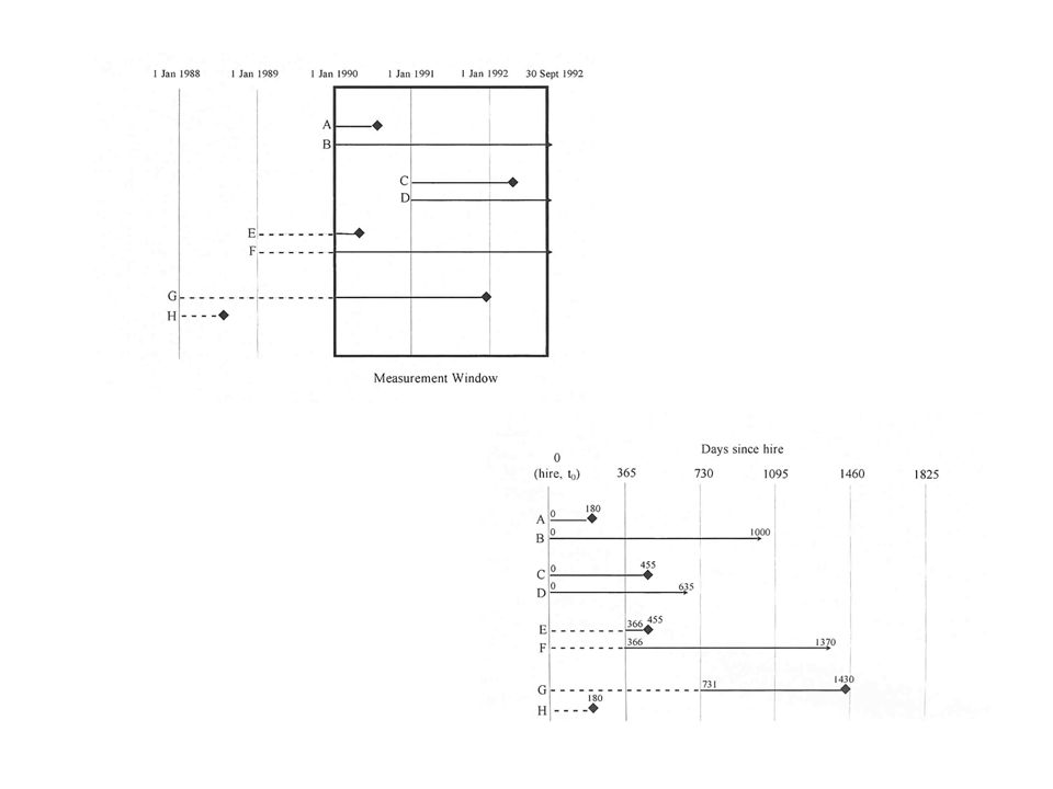
6. Example 1 Target population MDs who had service obligations in community health centers (to pay off loans) Interested in grads from 1988 on Goal is to find out if they became depressed Problem: We can not get a list of graduated physicians 03/2016 6

7. Example 1 (cont) Subject selection process (recruitment date) All MDs who worked in clinics between Jan 1, 1990 & Sept 30, 1992 Issue: Many MDs who graduated between 1988 and 1990 worked in clinics before recruitment started 03/2016 7

8. 8

9. Example 2 WHAS500 data set (used in Case Study #6) 500 people admitted to hospital with acute MI Interested in predictors of survival post MI BUT, only in people who were discharged alive from hospital Subject enters observation when they are discharged Follow-up starts on admission 03/2016 9

10. Example 2 (cont) If person died in hospital, they contribute no information to study If discharged alive, they contribute only after discharge. 03/2016 10

11. Left truncation (aka delayed entry) Subject ‘technically’ enters cohort at time ‘0’ Becomes ‘under observation’ is at later time ‘t’ Subject must be outcome free at this time If they had an event prior to this time, they never make it into the follow-up dataset Distribution of survival times is ‘truncated’ or ‘cut-off’ in the left tail 03/2016 11

12. Left truncation is more common when time scale is age Risk set is people of the same age People enter study at different ages Time ‘0’ is basically birth No information on outcomes from birth to age at entry AKA: Delayed entry 03/2016 12

13. Two ways of recruiting which give left truncation Prospective Recruit at time of eligibility (e.g.. diagnosis of cancer) Start observing after some future event (e.g. discharge from hospital). 03/2016 13

14. Two ways of recruiting which give left truncation (cont) Retrospective Identify subjects at time of some event in the future on the clinical or personal time line People discharged from hospital Determine eligibility by retrospective data collection Main difference is that truncated people never get identified by study in retrospective method 03/2016 14

15. Example 3 Study recruits 3,000 people discharged from hospital with history of heart disease Follow for two years to examine predictors of death But, age at diagnosis (eligibility) was up to 40 years earlier 03/2016 15

16. 03/2016 16 Two potential time ‘0’ points for standard analyses Date of CHD Dx Date of recruitment Death What to use as time ‘0’? Date of recruitment Date of Dx Both have problems

17. Suppose we use: Time ‘0’ = date of initial Dx We estimate survival from initial Dx S(t) is biased People with Dx prior to recruitment to study must have h(t) = 0 Immortal person time S(t) is an average of the ‘0’ hazard and the actual hazard. 03/2016 17

19. Suppose we use: Time ‘0’ = date of recruitment to study Measures survival post recruitment Ignores history prior to recruitment. Recruited groups contains people with varying pre- recruitment time with heart disease. All must have survived from Dx to recruitment date 03/2016 19

20. Time ‘0’ = date of recruitment to study (cont) S(t) is biased People with longer pre-recruitment Dx are in a more advanced stage of their follow-up Don’t represent survival experience for the period immediately after a person’s Dx S(t) is an average of different survival experiences at different points of post-Dx time/experience. 03/2016 20

21. 03/2016 21

22. 2 Solutions which give unbiased estimates Exclude patients from the study sample who were diagnosed prior to recruitment Date of recruitment = date of Dx  unbiased S(t) measure Causes a major drop in sample size 03/2016 22

23. 2 Solutions which give unbiased estimates Use an inception cohort Recruit people into study at date of Dx. Can be done prospectively But, can also do this ‘historically’ Define an entry date some time in the past Identify all newly diagnosed case after that date Determine predictors and outcomes Works best with a registry (e.g. cancer) 03/2016 23

24. No analytic method can recover information on events during the truncation period If we can ignore this, solution is ‘easy’ Set the ‘immortal person-time’ as outside the period of follow-up. Subjects have ‘delayed entry’ into study Assumes that the hazard starting from the time of recruitment is unaffected by the delayed entry 03/2016 24

25. Two approaches can be used in SAS. Define a delayed entry or truncation time variable Add a command to the Model statement giving entry time to risk set 03/2016 25

26. Two approaches can be used in SAS (cont) Use the Counting process input style Only one interval From entry time to end of study Need to specify (for each subject): Start of their follow-up time End of their follow-up time Outcome status (event vs. censored) No need to do any data re-structuring in this case 03/2016 26

27. Example #2 (cont) Want to estimate predictors of survival from time of MI for people who are discharged alive from hospital People dying in hospital are left truncated 03/2016 27

28. Example #2 (cont) Data set has a variable (LOS) which is the number of days in hospital Method 1: Add LOS to model statement as ‘entrytime’ Method 2: No need to rearrange data only one interval per subject starts at ‘LOS’ ends at study time 03/2016 28

29. 03/2016 29 proc phreg data = whas500A; model lenfol*fstat(0) = bmifp1 bmifp2 age hr diasbp gender chf age*gender/; run; proc phreg data = whas500A; model lenfol*fstat(0) = bmifp1 bmifp2 age hr diasbp gender chf age*gender/ entrytime = los; run; proc phreg data = whas500A; model (los,lenfol)*fstat(0) = bmifp1 bmifp2 age hr diasbp gender chf age*gender; run;

30. 03/2016 30 Ignores late entry

31. 03/2016 31 Late entry, method #1

32. 03/2016 32 Late entry, method #2