Download presentation
Presentation is loading. Please wait.

1
Digital Signal Processing Lecture 6 Frequency Selective Filters
بسم الله الرحمن الرحيم University of Khartoum Department of Electrical and Electronic Engineering Diploma/M. Sc. Program in Telecommunication and Information Systems Digital Signal Processing Lecture 6 Frequency Selective Filters Dr. Iman AbuelMaaly

2
Outlines LTI systems as frequency selective filters
Ideal filter characterisitics

3
LTI Systems as Frequency Selective Filters
An LTI system perform a filtering process among the various components at its input. An LTI system is a frequency shaping filter (or a frequency selective filter. Applications: Removal of undesirable noise Equalization of communication channels Signal detection in radar or sonar Spectral analysis of signals.

4
Ideal Filter Characteristics
Ideal filters include LPF – HPF – BPF – BSF Characteristics of ideal filters: These filters have a constant gain (unity gain) passband characteristics and zero gain in their stopband. Another characteristics of an ideal filters is a linear phase response.
 passband characteristics and zero gain in their stopband. Another characteristics of an ideal filters is a linear phase response")
5
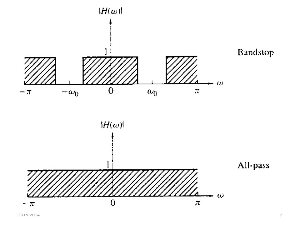
Ideal Filter Characteristics
Magnitude response for some ideal frequency –selective discrete time filters

8
Ideal Filter Characteristics
Ideal filters are of linear phase response: Filter output is a delayed and amplitude scaled version of the input signal. Ideal filters have linear phase characteristics within their passband that is, The derivative of phase has the units of delay,

9
Ideal Filter Characteristics
τg(ω) is the signal delay as a function of frequency, and is called envelop delay or group delay. If Θ(ω) is linear ( as ) = constant All frequency components of the input signal undergo the same time delay. Such filters are not physically realistic
 is the signal delay as a function of frequency, and is called envelop delay or group delay. If Θ(ω) is linear ( as ) = constant. All frequency components of the input signal undergo the same time delay. Such filters are not physically realistic")
10
Ideal Filter Characteristics
For Example: The ideal LP filter has an impulse response This filter is not causal and is unstable. i.e, physically unrealizable. Its frequency response can be approximated by a realizable filter.

11
Ideal Filter Characteristics
In the previous sections we presented a graphical method for computing the frequency response characteristics from the pole-zero plot. In the following sections the same approach can be used to design digital filters.

12
Ideal Filter Characteristics
The basic principle of the pole-zero placement is: to locate poles near points of the unit circle corresponding to frequencies to be emphasized, and to place zeros near the frequency to be deemphasized.

13
Ideal Filter Characteristics
Constraints: All poles inside the unit circle -> for stability. ( zeros to be placed anywhere) All complex poles and zeros are in conjugate leads to real coefficients.
 All complex poles and zeros are in conjugate leads to real coefficients")
14
Ideal Filter Characteristics
For a given pole-zero pattern the system function is as follows: b0 is the gain constant which is selected such that Where ω0 is a frequency in the pass band of the filter. Usually select N ≥ M so that the filter has more poles than zeros.

15
Low-pass, high-pass and band-pass filers
For LP filters : Poles near unit circle at points corresponding to low frequency near (ω=0) Zeros are near or at unit circle at points corresponding to high frequencies (near ω =π) For HP filter : The opposite
 Zeros are near or at unit circle at points corresponding to high frequencies (near ω =π) For HP filter : The opposite")
16
Im(z) Re(z) Unit Circle
 Re(z) Unit Circle")
17
X X O X O X O O X X X X O O X O X X X

18
Low-pass, high-pass and band-pass filers
Example: A single pole filter with system function If a =0.9, select G =1 - a to have unity gain at ω =0 At high frequencies, the gain is relatively small.

19
Low-pass, high-pass and band-pass filers
An addition of a zero will lead to a one pole one zero filter: In this case the magnitude of H2(ω) goes to zero at ω=π
 goes to zero at ω=π")
20
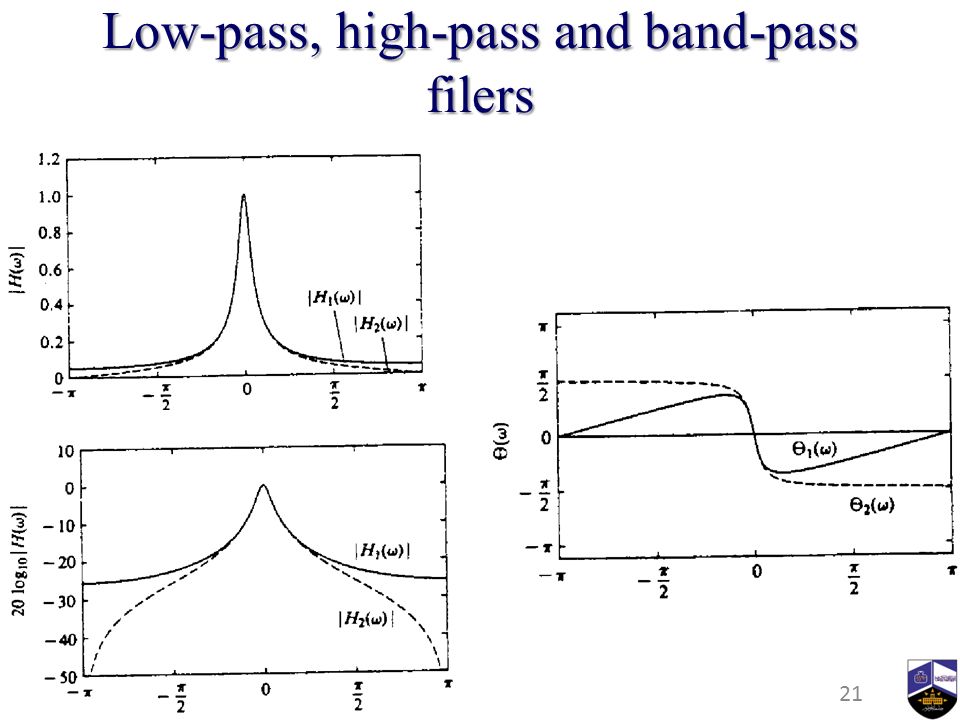
Low-pass, high-pass and band-pass filers
The figure below shows the magnitude and phase responses of A single pole filter, (2) A one pole-one zero filter;
 A one pole-one zero filter;")
21
Low-pass, high-pass and band-pass filers
22
Low-pass, high-pass and band-pass filers
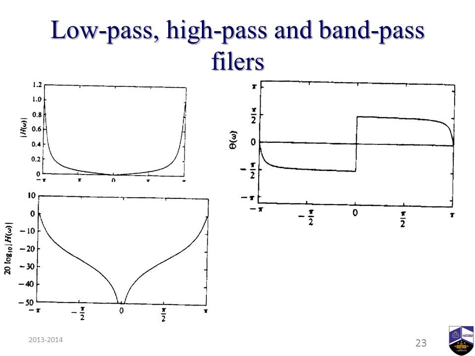
To obtain a high pass filter we reflect (fold) the pole-zero location of the LP filter about the imaginary axis in the z-plane. We obtain Its magnitude and frequency responses are shown below:
 the pole-zero location of the LP filter about the imaginary axis in the z-plane. We obtain. Its magnitude and frequency responses are shown below:")
23
Low-pass, high-pass and band-pass filers
24
Band Pass Filters The band pass filter should contain one or more pairs of complex conjugate poles near the unit circle, in the vicinity of the frequency band that constitute the pass band of a filter. Magnitude and phase response of a simple band pass filter are shown in the figure below:

25
Band Pass Filters

26
Band Pass Filters Example 2:
Design a two –pole filter that has the centre of its pass band at ω=π/2 .Zeros in its frequency response characteristics at ω=0 and ω=π and its magnitude is

27
A Simple Low Pass To High Pass Transformation
By using the frequency translation property of the Fourier transform, it is possible to convert the prototype filter to either a band pass filter, or a high pass filter. If is the impulse response of LTI is its frequency response A HP filter can be obtained by translating by π radians (replacing ω by ω- π )
")
28
A Simple Low Pass To High Pass Transformation
i.e., It can be proved that If the LP filter is described as follows difference equation Its frequency response is

29
A Simple Low Pass To High Pass Transformation
If we replace ω by ω- π, then: Which corresponds to

30
Examples Example 4.5.3

31
The Digital Resonator A digital resonator is a special two-pole BP filter with the pair of complex conjugate poles located near the unit circle. The name resonator refers to the fact that the filter has a large magnitude response (it resonates) in the vicinity of the pole location. The angular position of the pole determines the resonant frequency of the filter.
 in the vicinity of the pole location. The angular position of the pole determines the resonant frequency of the filter")
32
The Digital Resonator In the design of a digital resonator with a resonant peak at or near ω = ω0. We select the complex-conjugate poles at In addition, we can select up to two zeros. 1. One choice is a zero at z=1 and a zero at z=-1 Which eliminates the response of the filter at : ω = 0 and ω=π 2. The other choice is to locate zeros at the origin

33
The Digital Resonator Zeros are located at the origin
The system function with zeros at the origin is as follows: Since has its peak at or near ω = ω0, we select the gain b0 so that

34
The Digital Resonator We obtain Hence,
The desired normalization factor is

35
The Digital Resonator The frequency response can be expressed as:
Where U1(ω) and U2(ω) are the magnitude of the vectors from p1 and p2 to the point ω in the unit circle and Φ1(ω) and Φ2(ω) are the corresponding angles of these two vectors.
 and U2(ω) are the magnitude of the vectors from p1 and p2 to the point ω in the unit circle and Φ1(ω) and Φ2(ω) are the corresponding angles of these two vectors")
36
The Digital Resonator ωr is the resonant frequency of the filter.
For any value of r, U1(ω) takes its minimum value (1-r) at ω = ω0 The product U1(ω) U2(ω) reaches a minimum value at the frequency ωr. ωr is the resonant frequency of the filter.
 takes its minimum value (1-r) at ω = ω0. The product U1(ω) U2(ω) reaches a minimum value at the frequency ωr. ωr is the resonant frequency of the filter.")
37
The Digital Resonator The pole-zero pattern and a corresponding magnitude and phase response of a digital resonator with: (1) r =0.8 and (2) r = 0.95
 r =0.8 and (2) r =")
38
The Digital Resonator When r is close to the unity, ωr ≈ ω0 which is the angular position of the pole. As r approaches unity, the resonance peak becomes sharper because U1(ω) becomes more rapidly in relative size in the vicinity of ω0. A quantitative measure of the sharpness of the resonance is provided by the 3-dB bandwidth ∆ω of the filter. For value of r close to unity:
 becomes more rapidly in relative size in the vicinity of ω0. A quantitative measure of the sharpness of the resonance is provided by the 3-dB bandwidth ∆ω of the filter. For value of r close to unity:")
39
The Digital Resonator If the zeros are placed at z = ±1
The system function becomes And the frequency response

40
The Digital Resonator The zeros affect both the magnitude and phase of the resonator Where The addition of zeros leads to: A slightly smaller BW A very small shift in the resonant frequency due to presence of zeros.

41
The Digital Resonator The pole-zero pattern and a corresponding magnitude and phase response of a digital resonator with zeros at 1 and -1: (1) r =0.8 and (2) r = 0.95
 r =0.8 and (2) r =")
42
The Notch Filter It is a filter that contains one or more deep notches or, ideally, perfect nulls in its frequency response characteristics. Its applications are in case of some specific frequency components must be eliminated: Instrumentation and recording systems. Power line frequency of 60 Hz and its harmonics be eliminated.

43
The Notch Filter We need to create a null in the frequency response of the filter at ω0 . We simply introduce a pair of complex conjugate zeros on the unit circle at an angle ω0 , that is The system function of an FIR notch filter is

44
The Notch Filter Example: A notch filter with a null at Its magnitude response is as shown in the figure.
45
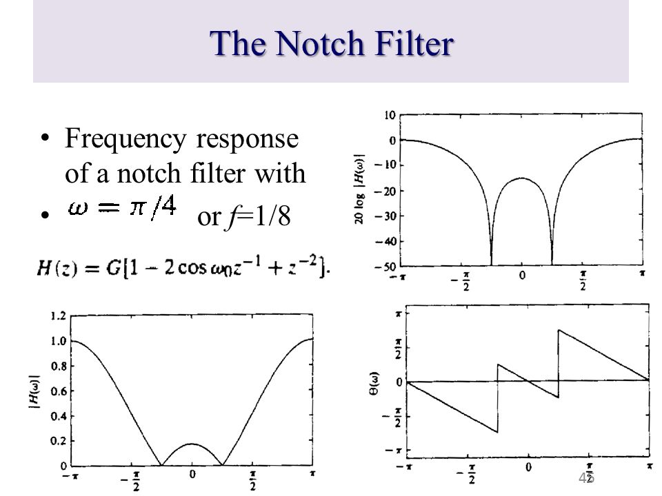
The Notch Filter Frequency response of a notch filter with or f=1/8
46
The Notch Filter The effect of poles is to reduce the BW of the notch.
The addition of poles near the null results a small ripple in the pass band of the filter due to the resonance created by the pole.

47
Notch Filters The figure below shows: the frequency response characteristics of two notch filters with poles at (1) r= 0.85 and (2) r=0.95
48
Note: r affect on notch tightness
Notch Filters Note: r affect on notch tightness

49
Next Lecture Frequency Selective Filters Cont.

Similar presentations


 can be.>")

 Kevin D. Donohue Electrical and Computer Engineering University of Kentucky.>")


