1. Advanced fMRI Methods John VanMeter, Ph.D. Center for Functional and Molecular Imaging Georgetown University Medical Center

2. Outline Arterial Spin Labeling (ASL) Diffusion –Diffusion Weighted Imaging (DWI) –Diffusion Tensor Imaging (DTI) –Incoherent Intravoxel Motion (IVIM) –Dynamic IVIM Functional Connectivity

3. Arterial Spin Labeling (ASL) Uses RF-pulse to “tag” spins in a slice Flowing blood moves from tagged slice up and through the arterial system Used to generate quantified resting blood flow maps and perform functional experiments

4. 90 0 RF Tagged 90 0 RF T=TE blood moves downstream flow direction vessel unsaturated spins unsaturated spins flipped out plane  flow void saturated spins saturated spins Spin Tagging

5. Radio Frequency Pulse to Tag Protons

6. ASL Sequence Acquire each slice twice: –one tagged and one untagged Subtract tagged from untagged to get slice with perfusion Using models of flow it is possible to quantify perfusion to obtain regional cerebral blood flow (rCBF)

7. Example Perfusion Images Brightness = rCBF

8. fMRI Using ASL vs. BOLD Detre, et. al, Clinical Neurophysiology 2002

9. ASL Results from Alcohol Study

10. ASL –Provides better spatial specificity –Not affected by “draining veins” –Less susceptible to scanner signal drift (useful for studies of changes that occur slowly over a long time scale) BOLD –Better temporal resolution –Better spatial resolution –MRI sequences readily available BOLD vs ASL

11. Diffusion KleenexNewspaper

12. Diffusion Weighted Imaging (DWI) Sequence Uses an EPI pulse sequence with bi-polar gradients applied during the sequence –First gradient disrupts the magnetic phases of all protons –Second gradient restores the phases of all stationary protons The restoration of signal is incomplete for protons that have moved (diffused) during the elapsed time

13. ADC (Apparent Diffusion Coefficient) non-linear fitting using image pixel values linear fitting using natural log of image pixel values b-value S    ln(S)   

14. Basic DWI Calculation Additional parameter in DWI is the b-value which defines both how strong the bi-polar gradients are and their duration Areas where diffusion occurs most rapidly will exhibit a greater decrease in MR signal as the b-value increases Collect multiple images each with a different b- value Typically estimated with just 2 b-values b-value ln S/S o

15. Apparent Diffusion Coefficient (ADC) Areas with higher rate of diffusion are brighter Little contrast between gray and white matter DWI calculation of ADC, relative rate of diffusion, is useful clinically (e.g. stroke ) Not of much use in research?

16. Diffusion Tensor Imaging (DTI) MR imaging technique in which contrast is based on both rate and direction in the diffusion of water molecules Because the cellular diffusion of water in the brain is limited by cell geometry, in particular axons, DTI can be used to examine the structure of white matter DTI used to identify and generate maps of white matter fibers

17. Diffusion Tensor Imaging DTI relates image intensities to the relative mobility of water molecules in tissue and the direction of the motion Motion of a water molecules is a random walk (Brownian motion) Areas with relatively high mean diffusion will appear dark on the Diffusion weighted MRI images

18. Types of Isotropy Anisotropic Isotropic KleenexNewspaper

19. Types of Isotropy In Vivo Open Pool of Fluid (Ventricles) Diffusion in an Axon

20. Models of 3D Isotropy Isotropic Anisotropic

21. DTI Sequence Repeat the DWI sequence with gradients applied in a number of different directions From the contribution of all the different directions we can calculate the direction of diffusion as well as the relative rate (ADC) Areas with restricted diffusion will have a directional bias which is used to determine the direction of diffusion

22. Raw Diffusion Images 6 directions Diffusion sensitive gradients applied in six directions all with b=1000 Dark areas represent areas with a higher degree of restricted diffusion

23. Different Gradient Directions 6 Directions 12 Directions 30 Directions

24. Diffusion Tensor Diffusion properties described with a 3 X 3 symmetric tensor matrix Diagonal elements of D (Dxx, Dyy, Dzz) are the ADC values along x, y and z axes respectively Off-diagonal elements (Dxy, Dxz, Dyz) represent the correlation between molecular displacements in orthogonal directions D

25. DTI Calculation Eigenvalues of the diffusion tensor ( x, y, and z ) provides length of the ellipsoid in the three principal directions of diffusivity Eigenvectors provide information about the direction of diffusion The eigenvector corresponding to the largest eigenvalue is used as the main direction of diffusion Maps are constructed of various measures of anisotropy from the eigenvalues and eigenvectors

26. Tensor Model of Isotropy IsotropicAnisotropic

27. Fractional Anisotropy (FA) Measure of degree of anisotropy regardless of direction Brighter areas correspond to areas with higher degree of anisotropic diffusion Ranges from 0 – 1 where FA=1 corresponds to completely anisotropic FA = ( x - y ) 2 + ( x - z ) 2 + ( y - z ) 2 2( x 2 + y 2 + z 2 )

28. Visualization of Direction of Diffusion Red = Left-Right Green = Anterior-Posterior Blue = Superior-Inferior

29. Structural Connectivity: Corpus Callosum Tracts

30. Diffusion Contrast & fMRI Diffusion in large blood vessels flows along direction of the vessel Diffusion in capillaries flows in multiple directions since each part of a capillary is oriented in different directions (more random motion) Applying diffusion gradients during BOLD acquisition can be used to eliminate signal from large vessels

31. Intravoxel Incoherent Motion (IVIM) BOLD measured with varying levels of diffusion weighting b=0 equivalent to regular BOLD Increasing b-values result in more restricted “activation” ADC map colors - red=large vessels blue=capillaries

32. Dynamic IVIM Acquire all of the diffusion data during fMRI paradigm Area of overlap taken as activation Advantages: high functional SNR and high spatial specificity

33. Functional Connectivity “Functional connectivity is defined as the correlations between spatially remote neurophysiological events” Friston, SPM Manual –Does not specify relationship between areas “Effective connectivity is the influence one neuronal system exerts over another” –Directionality of relationship is defined

34. Functional Connectivity During Condition X, both A & C activate During Condition Y, both B & C activate Since C is activated under both conditions but A and B are not, can infer directional relationships –A  C and B  C

35. Functional Connectivity Correlation is simplest method for computing functional connectivity –Time course of activity in one voxel is correlated against all other voxels –High correlations inferred to represent connectivity between regions Several other methods: –PCA (principal components analysis) –ICA (independent components analysis) –Structural Equation Modeling (SEM)

36. fMRI Example Stimuli 250 radially moving dots at 4.7 degrees/s Pre-Scanning 5 x 30s trials with 5 speed changes (reducing to 1%) 5 x 30s trials with 5 speed changes (reducing to 1%) Task - detect change in radial velocity Scanning (no speed changes) 6 normal subjects, 4 100 scan sessions; each session comprising 10 scans of 4 different condition e.g. F A F N F A F N S................. F - fixation point only A - motion stimuli with attention (detect changes) N - motion stimuli without attention S - no motion

37. Psychophysiological interactions: interactions: Attentional modulation of V2 -> V5 influences Attention V2 V5 attention no attention V2 activity V5 activity SPM{Z} time V5 activity

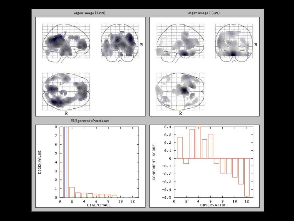
38. Y (DATA) time voxels Y = USV T = s 1 U 1 V 1 T + s 2 U 2 V 2 T +... use singular value decomposition (SVD) to determine: S (eigenvalues) U (eigenvariates, temporal) V (eigenvector, spatial) APPROX. OF Y U1U1 = APPROX. OF Y APPROX. OF Y + s 2 + s 3 +... s1s1 U2U2 U3U3 V1V1 V2V2 V3V3 PCA - Eigenimage Analysis

40. Minimise the difference between the observed (S) and implied () covariances by adjusting the path coefficients (a, b, c) The implied covariance structure: x= x.B + z x= z.(I - B) -1 x : matrix of time-series of regions U, V and W B: matrix of unidirectional path coefficients (a,b,c) Variance-covariance structure: x T. x =  = (I-B) -T. C.(I-B) -1 where C= z T z x T.x is the implied variance covariance structure  C contains the residual variances (u,v,w) and covariances The free parameters are estimated by minimising a [maximum likelihood] function of S and  Structural Equation Modeling (SEM) U W V a b c u v w

41. Attention - No attention Attention No attention 0.76 0.47 0.75 0.43