1. Tests of Significance We use test to determine whether a “prediction” is “true” or “false”. More precisely, a test of significance gets at the question of whether an observed difference is real or just a chance variation.

2. Example Suppose two investigators are arguing about a large box of numbered tickets. Null says the average is 50. (This number usually is obtained from experience or some other information.) But Alt says the average is different from 50. Both of them do not know how many tickets are there and what the average of the box is. So they agree to take a sample. The number of draws made at random is 500. The average of the sample turns out to be 48, and the SD is 15.3.

3. Example From the data, Null thinks that the difference is just 2, and the SD is 15.3. So the difference is so small relative to the SD, and it is just chance. What is wrong here? From the chapters of accuracy of inference we learned, we know that if we don’t know the composition of the box, we could use: The bootstrap procedure to make an estimation. But then the SD of the sample is very different from the SE for average.

4. Example

5. Comments There are two sides in this example: One side thinks a difference is real; the other side thinks the difference is just by chance. The latter side is beaten by a calculation. This calculation is called a test of significance. The key idea is that: if an observed value is too many SEs away from its expected value, then it is hard to explain by chance.

6. Terminologies In statistics, we have two hypotheses when doing test of significance: the null hypothesis and the alternative hypothesis. In the previous example: Null hypothesis: the average of the box equals 50. Alternative hypothesis: the average of the box is less than 50. The null hypothesis corresponds to the idea that an observed difference is due to chance. To make a test of significance, the null hypothesis has to be set up as a box model for the data. The alternative hypothesis is another statement about the box, corresponding to the idea that the observed difference is real. In general, the null hypothesis is set to be rejected.

7. Terminologies

8. In the previous example, we calculated the z-statistic ≈ -3. Alt says that 3 SEs below its expected value is quite a lot. Why is that? This is because of the normal curve: the area under the curve to the left of -3 is very small—about 1 in 1,000. That is the chance of getting a sample average 3 SEs or more below its expected value is about 0.1%. This 0.1% is called an observed significance level. The observed significance level is often denoted by P—for probability—and referred to as a P-value. In the previous example, the P-value of the test is about 0.1%.

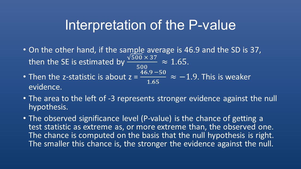
9. Interpretation of the P-value

11. Remarks As we seen, the test statistic z depends on the data, so does P. That is why P is called an observed significance level. We may see more clearly about the logic of the z-test: it is an argument by contradiction—to show the null hypothesis will lead to an absurd conclusion and must therefore be rejected. If we repeat the experiment of the test, the P-value tells us about the frequency of the time that our test statistics are as extreme as, or more extreme than the one we got before.(Think of multiple samples) This is another interpretation of the P-value, which is similar to the confidence intervals discussed before.

12. Remarks Remember, there is no way to define the probability of the null hypothesis being right. So the P-value is not the chance about the null hypothesis. No matter how often you do the draws, the box does not change. The null is just a statement about the box. The P-value of a test is the chance of getting a big test statistic— assuming the null hypothesis to be right. P is not the chance of the null hypothesis being right. The z-test is used for reasonably large samples, because of the normal approximation by CLT. With small samples, other techniques must be used.

13. Summary for making a test Set up the null hypothesis, in terms of a box model with tickets for the data. Pick a test statistic, draw the sample, measure the difference between the data from the sample and what is expected on the null hypothesis. Compute the observed significance level P-value.

14. Comments The choice of test statistic depends on the model and the hypothesis being considered. So far, we only have the “one-sample z-test”. Later on, we will discuss the “t-test”, the “two-sample z-test”, and the “χ²-test” if time permits. It is natural to ask how small the observed significance level has to be before we reject the null hypothesis. In general, we draw the line at 5%: If P is less than 5%, the result is called statistically significant (often shortened to significant). Another line is at 1%: If P is less than 1%, the result is called highly significant.

15. Questions Q: Do we have to strictly follow the lines? A: Need not. Do not let the jargon distract you from the main idea: the null hypothesis is rejected when the observed value is too many SEs away from the expected value. Q: In the previous example, for the alternative hypothesis, why we prefer “the average of the box is less than 50” rather than “more than 50”? A: This is due to the sample average 48. It becomes even worse if the average is more than 50. Q: When we do the z-test, what happen if z is positive? (For instance, suppose the sample average is 52 not 48.)

16. The test for counting problem The z-test can also be used when we have a problem about counting and classifying.

17. Example Charles Tart ran an experiment at the University of California, Davis, to demonstrate ESP (extrasensory perception). Tart used a machine to generate a number randomly, and the number will correspond to one of the 4 targets on the machine. Then the subject guesses which target was chosen, by pushing a button. The machine lights up the target it picked, ringing a bell if the subject guessed right.

18. Example Tart selected 15 subjects who were thought to be clairvoyant. Each of the subjects made 500 guesses. Out of the total 15 × 500 = 7,500 guesses, 2,006 were right. In general, the subjects will be right about ¼ of the time, whether or not they have the clairvoyant abilities. Then the expected correct guesses are ¼ × 7,500 = 1,875. The difference is 2,006 – 1,875 = 131 correct guesses. Tart use a test of significance to fend off the “it’s only chance”, in order to prove ESP.

19. Solution First, to set up a box model, Tart assume each of the 4 targets has 1 chance in 4 to be chosen. Tart assume (temporarily) that there is no ESP (null hypothesis), so that a guess has 1 chance in 4 to be right. By the assumption, the model is like the sum of 7,500 draws at random from the box with tickets: 1,0,0,0. (1 = right, 0 = wrong.) This completes the box model for the null hypothesis.

20. Solution

21. Comments There may be many reasonable explanations for the results, besides ESP. But chance variation is not one of them. The other possibilities to consider could be: For example, the random number generator of the machine may not be very good. Or the machine may be giving the subject some subtle clues as to which target it picked. The experiment may not prove ESP, but we know how the test of significance works.

22. Differences

23. The quantitative data is about the sum and the average. Then the SD has to be estimated. The qualitative data is about the number and percent. The SD is given by the composition. (counting and classifying) In the first example, there was an alternative hypothesis about the box: the average was below 50. Here, there is no sensible way to set up the alternative hypothesis. Reason: if the subjects do have ESP, the chance for each guess to be right may well depend on the previous trials, and may change from trial to trial. So the data will not be like draws from a box.

24. Differences In the first example, all the data were based on a box. All the arguments were based on the probability theory. Here, part of the question is whether the data are like draws from a box. If it were not, then it is not about the probability theory. In the last few chapters, we studied how to estimate parameters from data: averages, sums, numbers, and percentages. Here we learn how to test some arguments. Estimation and testing are related, but the goals are different.

25. Summary

26. The expected value is computed on the basis of the null hypothesis. If the null hypothesis determines the SD of the box, use this information when computing the SE. Otherwise, you have to estimate the SD from the data. The observed significance level, the P-value, is the chance of getting a test statistic as extreme as or more extreme than the observed one. The chance is computed on the basis that the null hypothesis is correct. The P-value is not the chance of the null hypothesis being right. Small values of P are evidence against the null hypothesis: they indicate something besides chance was operating to make the difference.