1. Environmental and Exploration Geophysics I tom.h.wilson wilson@geo.wvu.edu Department of Geology and Geography West Virginia University Morgantown, WV Resistivity II

2.  sourcesink 20m 12m  4m 2m Lets take a look at Problem 1 from Chapter 5 and take time for some questions. What kind of an array is this? What are d 1, d 2, d 3 and d 4 ? P1P1 P2P2 Find the potential difference between points 1 and 2.

3. The critical point here is that you accurately represent the different distances between the current and potential electrodes in the array. Use basic equations for the potential difference.

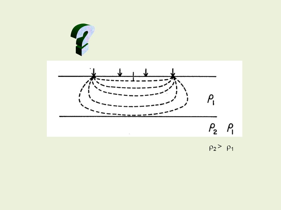
4. Current refraction rules Given these resistivity contrasts - how will current be deflected as it crosses the interface between layers? Measure the incidence angle and compute the angle of refraction.

6. tan  increases with increasing angle What’s your guess?  2 >  1  2 <  1

7. 11 22  2 varies as  1 and  1 varies as  2  2 >  1

9.  2 <  1

10.  2 >  1

11. Incorporating resistivity contrasts into the computation of potential differences. Let’s consider the in-class problem handed out to you last lecture.

12. Current reflection and transmission d1d1 d 2 = a+b  1 =30  -m  2 =350  -m Image point a b PAPA PBPB PCPC  One potential electrode Source Electrode Sink

13. In-Class Problem 2 In the preceding diagram - Suppose that the potential difference is measured with an electrode system for which one of the current electrodes and one of the potential electrodes are at infinity. Assume a current of 0.5 amperes, and compute the potential difference between the electrodes at P A and . Given that d 1 = 50m, d 2 = 100m,  1 = 30  -m, and  2 = 350  -m.

14. d1d1 d 2 = a+b  1 =30  -m  2 =350  -m Image point a b PAPA PAPA PAPA Reflection point Some current will be transmitted across this interface and a certain amount of current (k) will be reflected back into medium 1. ? At P A

15. Use of the image point makes it easy to estimate the length along the reflection path Path length is distance from image point to P A.

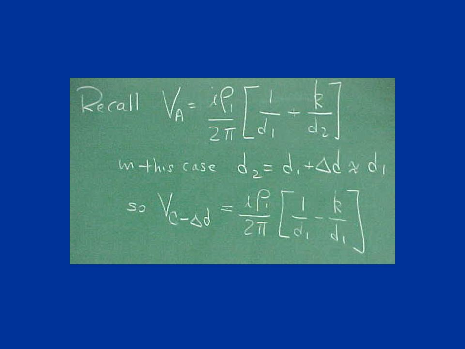
16. Potential measured at A k is the proportion of current reflected back into medium 1. k is also known as the reflection coefficient.

17. Potential measured at point B 1-k is the transmission coefficient or proportion of current incident on the interface that is transmitted into medium 2.

18. Potential measured at point C

21. Potentials a hair to the left or right of the interface should be approximately equal.

22. Incorporating resistivity contrasts into the computation of potential differences. Locate an image electrode and incorporate reflection process,

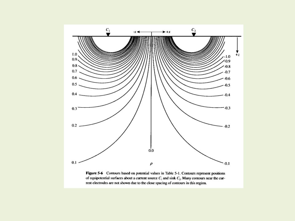
23. General ideas about potential field and current distributions.

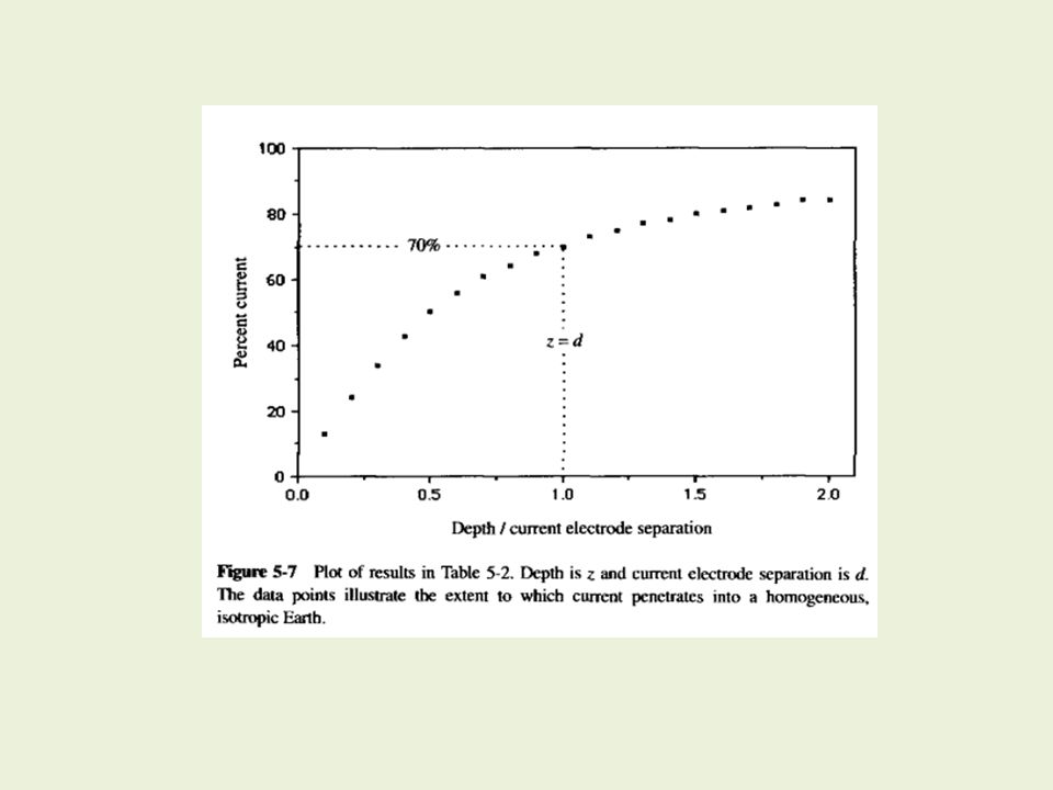
25. From the text we are given - z is depth and d is electrode spacing

27. In the preceding diagram z was depth. In this diagram z is depth divided by a which is 1/3 rd the current electrode separation.

28. Note the similarity of this “sensitivity” curve to the relative response function (  V (z)) used with terrain conductivity data. You can also think of this curve as indicating the contribution of intervals at various depths to the potential between one current and one potential electrode.

29. We see that in general for the Wenner array the peak sensitivity of the array to subsurface resistivity distributions occurs at depths approximately equal to the a-spacing.

30. By comparison to the characterization of instrument response as a function of depth and intercoil spacing these relationships are defined much more qualitatively for the resistivity applications.

31. How many layers have been sensed in this resistivity sounding? Qualitative interpretation of a resistivity sounding - The observations consist of apparent resistivities recorded at various a-spacings (Wenner array) or l-spacings (Schlumberger array). See empirical methods on pages 95 and 296 of Berger.

32. There are several ways to envision the relationship between measured apparent resistivity and subsurface resistivity distributions. A parallel circuit relationship has been suggested.

33. The determination of depth to resistivity boundaries has been suggested to be related to breaks in the cumulative resistivity plot. What is the Depth to a resistivity boundary?

34. Let’s examine the utility of some of these “rules-of-thumb” using synthetic data. Synthetic data are data that have been calculated from a model. Thus we know what the actual answer should be. Given the potential how do we determine apparent resistivity?

35. The apparent resistivities (  a ) are computed from the relationship we derived earlier. Where G = 2  a for the Wenner array

36. Here are some plots of our synthetic or “test” data set. The model from which it is derived is shown at lower right.

37. The Inflection Point Depth Estimation Procedure This technique suggests that the depths to various boundaries are related to inflection points in the apparent resistivity measurements. Again, the In-Class data set illustrates the utility of this approach. Apparent resistivities plotted below are shown over the model for both the Schlumberger and Wenner arrays. The inflection points are located, and dropped to the spacing-axis. The technique is suggested too be most applicable for use with the Schlumberger array. A common rule would be that the depth to the top of the high resistivity layer encountered in this survey would be equal to inflection point l-spacing divided by 2. For the Schlumberger array this would give a depth to the top of the layer of about 12 meters instead of the actual depth of 8. This rule actually works better for the Wenner array. In the case of the Wenner array we would get a depth of about 9 meters. I suggest that a better “rule of thumb” for the Schlumberger array would to divide the inflection point distance by 4 (or even 3) instead of 2.

38. Resistivity determination through extrapolation This technique suggests that the actual resistivity of a layer can be estimated by extrapolating the trend of apparent resistivity variations toward some asymptote, as shown in the figure below. The problem with this is being able to correctly guess where the plateau or asymptote actually is. Spacings in the In-Class data set only go out to 50 meters. The model data set (below) used for the inflection point discussion reveals that this asymptote is reached only gradually, in this case at distances of 500 meters and greater. Since most of the layers affecting the apparent resistivity in our surveys will be associated with thin layers, we are unlikely to be able to do this very accurately. The apparent resistivity will vary considerably over that distance rather than rise gradually to resistivities of individual layers. At best the technique offers only a crude estimate.

39. Moores Cumulative Resistivity Technique This technique suggests that the sum of the apparent resistivities when measured at constant intervals of a (i. e., 5, 10, 15, 20,..., not 1,2,4,6,10,20....) will yield linear segments whose intersection points mark layer boundaries. If you recall from lecture, this idea assumes that apparent resistivities are constant when a-spacings and therefore maximum sensitivities are within a given layer. Remember that the zone of maximum sensitivity lies at a depth z=a. However, the figure below reveals a pitfall in this technique. The apparent resistivities are relatively constant out to a-spacings of about 6 meters, but begin to rise as the zone of maximum sensitivity extends down into the layer beneath. This transition takes place over a large range of a-spacings, extending from 6 meters out to 500 meters before flattening out at the 139  -m resistivity of the deeper layer. On the two flat segments, 0-6 meters and 500 to  the response is flat, and the slope of the sum be constant. Between 6 and 500 meters the slope of the sum will gradually increase before reaching the next linear segment.

41. Summary - Barnes Parallel Resistor Method Apparent resistivity is assumed to be a combination of resistances in parallel, i.e.,  1 is assumed to equal the apparent resistivity at the shortest a-spacing. The technique does not yield very realistic answers. I have found no good examples of its use, just textbook descriptions. Trying it on the class example illustrates the use of the technique. If you simply solve  for successive measurements of  a, you get an additional layer for each measurement, and the resistivities show up pretty far from the barn (see Figure at right). Our interpretation tells us we have a two-layer problem. RESIXIP resolves 2 layers; one, near- surface with  = 20  -m, and a deeper layer (top at about 8 meters) with a   139  -m. If you ask “What should  a2 be so that  2 = 139?” then you find that  a2 must =23.36  -m. I find it impossible to come up with means of picking this number (23.36  -m) from the observed resistivity data.

42. MORAL: Beware of the Barn.

43. Method of Characteristic curves The curves are calculated responses for given conditions. The curves shown at right are for a two-layer model. We’ll consider this method in more detail during lecture next Thursday.

44. Equivalence - non-uniqueness...

45. The realm of possibility...

46. Multi-electrode resistivity systems

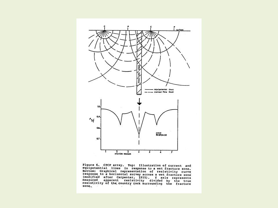
48. Tri-potential resistivity method

49. Normal Wenner array configuration

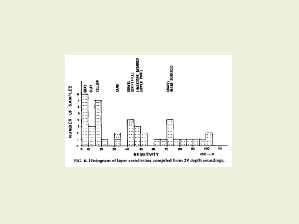
58. Some background information about the resistivity lab

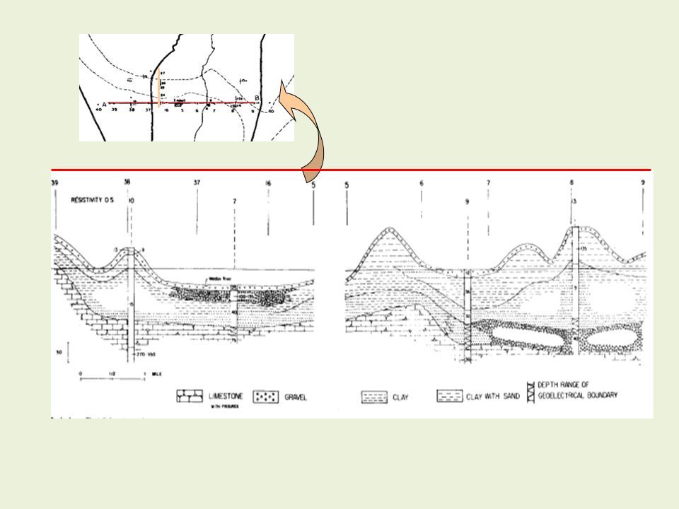
62. Frohlich used the method of characteristic curves to estimate the depths to resistivity interfaces and their resistivity. We’ll talk more about the method of characteristic curves in the next lecture.

63. Hand in problems 1-3 next class. Read over Frohlich’s paper before next Tuesday’s lab Next Class