Download presentation
Presentation is loading. Please wait.

2
Properties of Open Channels Free water surface Position of water surface can change in space and time Many different types River, stream or creek; canal, flume, or ditch; culverts Many different cross-sectional shapes

3
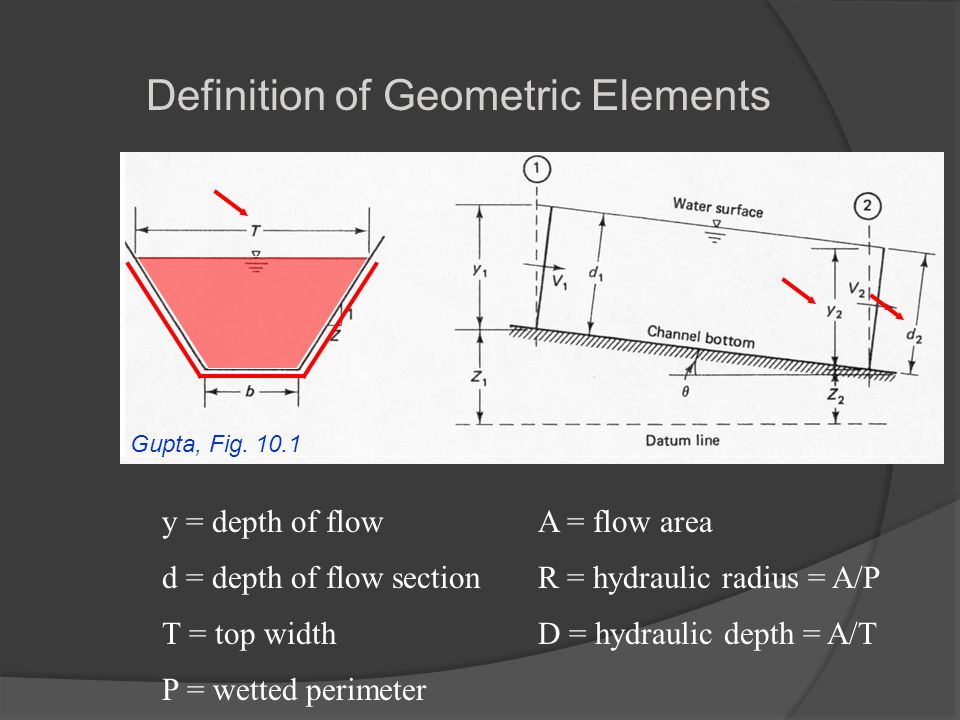
Definition of Geometric Elements R = hydraulic radius = A/P D = hydraulic depth = A/T y = depth of flow d = depth of flow section T = top width P = wetted perimeter A = flow area Gupta, Fig. 10.1
4
Circular Sections For partially full circular sections (with diameter d o ), the geometric elements are a function of depth (y) Values have been tabulated in non- dimensional form using d o as a scaling parameter (Gupta Table 10.1) Note that maximum flow occurs at a depth of 0.94d o
, the geometric elements are a function of depth (y) Values have been tabulated in non- dimensional form using d o as a scaling parameter (Gupta Table 10.1) Note that maximum flow occurs at a depth of 0.94d o")
5
Geometric Elements for Circular Pipes Gupta, Table 10.1

6
Flow Classification Uniform (normal) flow: Depth is constant at every section along length of channel Nonuniform (varied) flow: Depth changes along channel Rapidly-varied flow: Depth changes suddenly Gradually-varied flow: Depth changes gradually
 flow: Depth is constant at every section along length of channel Nonuniform (varied) flow: Depth changes along channel Rapidly-varied flow: Depth changes suddenly Gradually-varied flow: Depth changes gradually")
7
State of Flow Flow in open channels is affected by viscous and gravitational effects Viscous effects described by Reynolds number, Re = VR/ Gravitational effects described by Froude number, F = V/(gD) 1/2
 1/2")
8
Viscous Effects For Re < 500, viscous forces dominate and flow is laminar For Re > 2000, viscous forces are weak and flow is turbulent For Re between 500 and 2000, there is a transition between laminar and turbulent flow

9
Gravitational Effects Critical flow is the point where velocity is equal to the speed of a wave in the water For F = 1, flow is critical For F < 1, flow is subcritical Wave can move upstream For F > 1, flow is supercritical Wave cannot move upstream

10
Equations of Motion There are three general principles used in solving problems of flow in open channels: Continuity (conservation of mass) Energy Momentum For problems involving steady uniform flow, continuity and energy principles are sufficient
 Energy Momentum For problems involving steady uniform flow, continuity and energy principles are sufficient")
11
Conservation of Mass Since water is essentially incompressible, conservation of mass (continuity) reduces to the following: discharge in = discharge out Stated in terms of velocity and area: Q = V 1 A 1 = V 2 A 2 (10.5)
 reduces to the following: discharge in = discharge out Stated in terms of velocity and area: Q = V 1 A 1 = V 2 A 2 (10.5)")
12
Control Volume for Open Channels Gupta, Fig. 10.4

13
Conservation of Energy Conservation of energy applied to control volume results in the following: whereZ 1,Z 2 are elevations of the bed, y 1, y 2 are depths of flow, V 1, V 2 are velocities, 1, 2 are kinetic energy corrections, and h f is the frictional loss.

14
Energy Coefficient The term associated with each velocity head ( ) is the energy coefficient This term is needed because we are using the average velocity over the depth to compute the total kinetic energy Integrating the cubed incremental velocities is not equal to the cube of the integrated incremental velocities
 is the energy coefficient This term is needed because we are using the average velocity over the depth to compute the total kinetic energy Integrating the cubed incremental velocities is not equal to the cube of the integrated incremental velocities")
15
Critical Flow Specific energy is defined as the energy in a channel section measured w.r.t. channel bed If slope of channel is relatively flat, we can let Z 1 = Z 2 = 0 For energy coefficient ( ) = 1, specific energy (E) is thus
 = 1, specific energy (E) is thus.")
16
Specific Energy Gupta, Fig. 10.7

17
Critical Depth The point of minimum specific energy corresponds to the critical depth For higher values of specific energy there are two values that give the same specific energy If Q is fixed, for the smaller depth there will be a higher velocity (supercritical) and for the larger depth there will be a lower velocity (subcritical)
 and for the larger depth there will be a lower velocity (subcritical)")
18
Computing Critical Flow From necessary condition for minimum specific energy, can define section factor for critical flow (Z c ): whereZ c is the critical section factor, A is the area of flow, D is the hydraulic mean depth, and Q is the discharge
: whereZ c is the critical section factor, A is the area of flow, D is the hydraulic mean depth, and Q is the discharge")
19
Computing Critical Flow If y c is known, can compute Z c for specific geometry. Then critical discharge is given as

20
Computing Critical Depth If Q is known, can compute Z c as For simple geometries, Z c can be written as a function of y c (see Example 1) For complex geometries, use tabulated values (see Example 2)
 For complex geometries, use tabulated values (see Example 2)")
21
Example 1 Determine the specific energy of water in a rectangular channel 25 ft wide having a flow of 500 cfs at a velocity of 5 ft/s. What is the critical depth of water in the channel? What is the critical velocity?

22
Example 2 Determine the specific energy of water in the trapezoidal channel shown having a flow of 30 m 3 /s. What is the critical depth of water in the channel? What is the critical velocity? 4m 4 1 y

23
Uniform Flow Equations are developed for steady- state conditions Depth, discharge, area, velocity all constant along channel length Rarely occurs in natural channels (even for constant geometry) since it implies a perfect balance of all forces Two general equations in use: Chezy and Manning formulas
 since it implies a perfect balance of all forces Two general equations in use: Chezy and Manning formulas")
24
Chezy Equation Balances force due to weight of water in direction of flow with opposing shear force Note: V is mean velocity, R is hydraulic radius (area/wetted perimeter), S is the slope of energy gradeline, and C is the Chezy coefficient C is a function of the roughness of the channel bottom
, S is the slope of energy gradeline, and C is the Chezy coefficient C is a function of the roughness of the channel bottom")
25
Manning Equation The Manning equation is an empirical relationship similar to Chezy equation: Note: V is mean velocity (ft/s), R is hydraulic radius (ft), S is the slope of the energy gradeline (ft/ft), and n is the Manning roughness coefficient
, R is hydraulic radius (ft), S is the slope of the energy gradeline (ft/ft), and n is the Manning roughness coefficient")
26
Manning Equation The Manning equation for metric units is given as: Note: V is mean velocity (m/s), R is hydraulic radius (m), S is the slope of the energy gradeline (m/m), and n is the Manning roughness coefficient
, R is hydraulic radius (m), S is the slope of the energy gradeline (m/m), and n is the Manning roughness coefficient")
27
Manning ’ s Roughness (n) Roughness coefficient (n) is a function of: Channel material Surface irregularities Variation in shape Vegetation Flow conditions Channel obstructions Degree of meandering
 Roughness coefficient (n) is a function of: Channel material Surface irregularities Variation in shape Vegetation Flow conditions Channel obstructions Degree of meandering")
28
Manning’s n Gupta, Table 10.6

29
Manning ’ s Equation Using continuity equation (Q=VA), Manning’s equation for English units can be written as And for metric units
, Manning’s equation for English units can be written as And for metric units")
30
Conveyance For uniform flow, A, R and n are constant thus The term K is conveyance, given as

31
Normal Section Factor Based on Manning’s equation, define a normal section factor for the portion dependent on geometry, namely For simple geometries, Z n can be written as a function of y n For complex geometries, use tabulated values (e.g., Gupta Table 10.1)
")
32
Computing Normal Flow Three cases to consider: Ê Find Q for known values of y n and S Ë Find S for known values of Q and y n Ì Find y n for known values of Q and S From Manning’s equation, see that

33
ÊComputing Normal Flow For known values of y n and S, can use Manning’s equation directly Based on relationship between y n and Z n, determine the value of Z n Compute discharge from Manning’s equation, namely

34
Example 3 Calculate the discharge through a 3-ft diameter circular clean earth channel running half full. The bed slope is 1 in 4500. Manning’s n = 0.018.

35
ËComputing Normal Slope For known values of y n and Q, can use Manning’s equation directly Based on relationship between y n and Z n, determine the value of Z n Rearrange Manning’s equation, and compute slope as

36
Ì Computing Normal Depth For known values of Q and S, can compute Z n as Normal depth (y n ) is then determined from the relationship between y n and Z n
 is then determined from the relationship between y n and Z n")
37
Example 4 A trapezoidal channel flowing at 30 m 3 /s has a bottom slope of 0.1% and n = 0.025. Determine the normal depth. Determine the critical slope. What is the state of flow in the channel? 4m 4 1 y

38
Alterations to the HGL As with pipes, there are numerous structures and channel alterations that affect the hydraulic grade line (HGL). These alterations result in minor losses. We will consider 5 cases: Sudden transitions Constrictions and obstructions Junctions Trash Racks Gates

39
Sudden Transitions Changes in cross-sectional geometry over a short distance results in rapidly varied flow This can produce a sharp drop (contraction) or rise (expansion) of the HGL Change in geometry can be in either the horizontal or vertical plane of the channel
 or rise (expansion) of the HGL Change in geometry can be in either the horizontal or vertical plane of the channel")
40
Horizontal Contractions Writing the momentum and continuity equations between sections 1 and 3 and neglecting frictional losses and the momentum correction factor: where Source: Chow (1959) Figure 17-3
 Figure 17-3")
41
Horizontal contractions/expansions The equation can be plotted against y 3 /y 1 using b 3 /b 1 as a parameter Source: Chow (1959) Figure 17-2
 Figure 17-2")
42
Horizontal contractions/expansions For a given expansion (b 3 /b 1 > 1) or contraction (b 3 /b 1 < 1), the curves can be used to solve for y 3 given Q and y 1 : Compute F 1 2 from Q and y 1 Use curves to determine y 3 /y 1 To determine y 1 given Q and y 3 : Assume a value of y 1 Compute {F 1 2 } Use curves to determine F 1 2 using y 3 /y 1 and b 3 /b 1 Iterate on value of y 1 until {F 1 2 } = F 1 2
 or contraction (b 3 /b 1 < 1), the curves can be used to solve for y 3 given Q and y 1 : Compute F 1 2 from Q and y 1 Use curves to determine y 3 /y 1 To determine y 1 given Q and y 3 : Assume a value of y 1 Compute {F 1 2 } Use curves to determine F 1 2 using y 3 /y 1 and b 3 /b 1 Iterate on value of y 1 until {F 1 2 } = F 1 2")
43
The drop in the EGL for a contraction or expansion can be calculated as Horizontal contractions/expansions

44
Sudden Transitions Based on the resulting values of F 1 2 and F 3 2, the transitions fall into four possible cases: Region 1: F 1 2 <1, F 3 2 <1 ○ Flow is supercritical throughout the transition Region 2: F 1 2 1 ○ Flow through the transition passes from supercritical to subcritical (hydraulic jump) Region 3: F 1 2 >1, F 3 2 >1 ○ Flow is subercritical throughout the transition Region 4: F 1 2 >1, F 3 2 <1 ○ Flow through the transition passes from subcritical to supercritical
 Region 3: F 1 2 >1, F 3 2 >1 ○ Flow is subercritical throughout the transition Region 4: F 1 2 >1, F 3 2 <1 ○ Flow through the transition passes from subcritical to supercritical")
45
Constrictions and Obstructions For drastic constrictions of the channel area (b 3 /b 1 < 0.8), the calculations and resulting water-surface profiles are complicated Likewise, calculating the effect of obstructions (e.g., piers) involves sophisticated calculations These problems are generally solved using step-backwater computational software (e.g., U.S. Army Corps of Engineers HEC- RAS software), and are beyond the scope of this class
, and are beyond the scope of this class.")
46
Junctions Understanding flow through channel junctions involves numerous variables, such as number of channels, angles of intersection, cross-sectional shape and slope of the channels, directions of flow, etc. Theoretical solutions have only been determined for simple cases. More complex situations are usually solved using numerical techniques applied to a branching flow network

47
Special case: Combining Flow For the special case of a rectangular channel flowing into an equal-sized rectangular channel, applying the momentum equation results in 1 3 2 yuyu ydyd

48
Special case: Combining Flow If we know the flow in the two joining channels (Q 1 and Q 2 ), assuming normal flow upstream of the junction results in values for y 1 and y 2. From continuity, Q 3 = Q 1 +Q 2 Setting y u =y 1, we can solve for y d using an iterative solution: Assume a value for y d Calculate LHS from known quantities Calculate RHS for assumed y d Iterate until LHS = RHS

49
Trash Racks Head loss through trash racks can be computed using the standard minor loss equation The minor loss coefficient (K t ) is a function of the bar thickness (s), distance between bars (b), bar shape and the angle of the rack from the horizontal plane ( )
 is a function of the bar thickness (s), distance between bars (b), bar shape and the angle of the rack from the horizontal plane ( )")
50
Trash Racks The shape factor ( ) is tabulated based on the shape of the bar More sophisticated equations for the minor loss coefficient are available for racks that aren’t perpendicular to the flow in the channel Form of rack bar Shape factor ( ) Square nose and tail2.42 Square nose, semicircular tail1.83 Semicircular nose and tail1.67 Round1.79 Airfoil0.76
 is tabulated based on the shape of the bar More sophisticated equations for the minor loss coefficient are available for racks that aren’t perpendicular to the flow in the channel Form of rack bar Shape factor ( ) Square nose and tail2.42 Square nose, semicircular tail1.83 Semicircular nose and tail1.67 Round1.79 Airfoil0.76")
51
Gates Gates can be used to control the flow in a channel or at the entrance from a reservoir to a channel The sluice and tainter gates are common underflow structures The design typically involves estimating the discharge rating of the structure for various gate opening heights and upstream water- surface elevations

52
Underflow Gates For both styles of gates, the energy equation can be solved to give the following rating: Source: Chow (1959) Figure 17-37 length upstream depth discharge coefficient gate opening
 Figure length upstream depth discharge coefficient gate opening")
53
Vertical sluice gates The discharge coefficient is a function of the upstream depth, sluice opening, and downstream depth Source: Chow (1959) Figure 17-38 submerged conditions y 3 /h > 2
 Figure submerged conditions y 3 /h > 2")
54
Tainter gates The discharge coefficient for a tainter gate is more complicated, and depends on the radius of the gate (r) and the location of the pivot point (a) Source: Chow (1959) Figure 17-39 submerged conditions
 and the location of the pivot point (a) Source: Chow (1959) Figure submerged conditions")
55
Channel Design Previously, we have assumed that channel dimensions and slope are known In design situations, usually know discharge and need to determine geometry and slope In an open channel, usually have allowable velocity range Minimum of 2-3 ft/s to move grit Maximum velocity to prevent scouring

56
Channel Design For circular pipes, can determine minimum slope needed to achieve a minimum velocity of 2 ft/s Gupta, Table 10.7

57
Channel Design From basic principles, we know that: For a given slope and roughness, Q increases with increase of section factor (Z n =AR 2/3 ) For a given area, Z n is maximum for a minimum wetted perimeter (P) Based on these principles, can develop guidelines for efficient hydraulic sections for given channel shapes
 For a given area, Z n is maximum for a minimum wetted perimeter (P) Based on these principles, can develop guidelines for efficient hydraulic sections for given channel shapes")
58
Efficient Hydraulic Sections

59
Design Procedure For a specified Q, select S and estimate Manning’s n. Compute section factor from Q, n and S Select a shape, and express section factor in terms of y; solve for y Try different values of S, n and shape and compute cost for each Verify that velocity exceeds 2-3 ft/s Add freeboard if open section

Similar presentations


 Chapter 9: FLOWS IN PIPE>")


