1. 1 Chapter 3 Digital models of speech signal

2. 2 Introduction In order to apply digital signal processing technique to speech processing problems, it is essential to understand the fundamentals of the speech production process as well as digital signal processing. This chapter provides a review of acoustic theory of speech production and shows how this theory leads to a variety of ways of representing of the speech signal.

3. 3 Introduction This chapter begins with a very brief introduction to acoustic phonetics, a discussion of the place and manner of articulation for each of the major phoneme classes. Then the fundamentals of the acoustic theory of speech production are presented which include Sound propagation in the vocal track Transmission line analogies Steady state behavior of the vocal system.

4. 4 3.1 The process of speech production Speech signals are composed of a sequence of sounds. These sounds and the transitions between them serve as a symbolic representation of information. The arrangement of these sounds is governed by the rules of language. The study of these rules and their implications in human communication is the domain of linguistics. The study and classification of the sounds of speech is called phonetics.

5. 5 3.1.1 The mechanism of speech production The vocal track begins at the opening between vocal cords or glottis and end at the lips, consist of pharynx. Vocal length of male=17cm Cross-sectional area varies from 0 to 20 cm 2. The nasal track begins at the velum and ends at the nostrils.

6. 6 3.1.1 The mechanism of speech production The sub-glottal system serves as a source of energy for the production of speech. Speech: Radiated wave from the system when air is perturbed by a constriction somewhere in the vocal track.

7. 7 3.1.1 The mechanism of speech production Speech sounds can be classified into 3 distinct classes according to their mode of excitation. 1. Voiced sound: Produced by forcing air through the glottis with the tension of the vocal cords adjusted so that they vibrate in a relaxation oscillation, thereby producing quasi-periodic pulses of air which excite the vocal track. Example: U, d, w, i, e.

8. 8 3.1.1 The mechanism of speech production 2. Fricative or unvoiced sounds: Generated by forming a constriction at some point in the vocal track and forcing air through the constriction at a high enough velocity to produce turbulence. This creates a broad-spectrum noise source to excite the vocal track. 3. Plosive sounds: Results from making a complete closure, building up pressure behind the closure, and abruptly releasing it.

9. 9 3.1.1 The mechanism of speech production

10. 10 3.1.1 The mechanism of speech production The vocal track and the nasal track are tubes of non-uniform cross-sectional area. As sounds propagates through these tubes, the frequency spectrum is shaped by the frequency selectivity of the tube. ( similar to resonance frequency). The resonance frequency of the vocal track tube are called formant frequencies or formants. Formants depend on the shape and dimension of the vocal track; each shape is characterized by a set of formant frequencies.

11. 11 3.1.1 The mechanism of speech production The time varying spectral characteristics of speech signal can be graphically displayed through the use of sound spectrograph. The device produces a two dimensional pattern called a spectrogram in which the vertical dimension corresponds to frequency and the horizontal dimension to time. The darkness of the pattern is proportional to signal energy. Voiced regions are characterized by a striated appearance due to the periodicity spectrogram.

12. 12 3.1.2 Acoustic phonetics Most language including English, can be described in terms of a set of distinctive sounds or phonemes. American language has 42 phonemes including vowels, diphthongs, semivowels and consonants. Continuant sound: Produced by a fixed vocal track configuration excited by the appropriate source. Vowels, fricatives and nasals. Non-continuant sound: Produced by a changing vocal track configuration.

13. 13 3.1.2 Acoustic phonetics

14. 14 3.1.2a Vowels Vowels are produced by exciting a fixed vocal track with quasi-periodic pulses of air caused by vibration of the vocal cords. The dependence of cross-sectional area upon distance along the track is called the area function of the vocal track. Example: a in father, I in eve.

15. 15 3.1.2a Vowels

16. 16 3.1.2a Vowels

17. 17 3.1.2a Vowels

18. 18 3.1.2a Vowels

19. 19 3.1.2b Diphthongs A diphthong is a gliding monosyllabic speech item that starts at or near the articulatory position for one vowel and moves to or forward the position for another. Diphthongs are produced by varying the vocal tract smoothly between vowel configurations appropriate to diphthongs.

20. 20 3.1.2b Semivowels The group of sounds consisting of w,l,r,y are called semivowels because of their vowel like nature. They are generally characterized by a gliding transition in vocal tract area function between adjacent phonemes.

21. 21 3.1.2C Nasals The nasal consonants are produced with glottal excitation and the vocal tract totally constricted at some point along the oral passage way. The velum is lowered so that air flows through the nasal tract, with sound being radiated at the nostrils.

22. 22 3.1.2d Nasals

23. 23 3.1.2e Unvoiced Fricatives The unvoiced fricatives f,θ,s and sh are produced by exciting the vocal tract by a steady air flow which becomes turbulent in the region of a constriction in the vocal tract. The location of the constriction serves to determine which fricative sound is produced.

24. 24 3.1.2f Voiced Fricatives The voiced fricatives v,th, z and zh are the counterparts of the unvoiced fricatives. The vocal tract are vibrating and thus one excitation source are is at the glottis.

25. 25 3.1.2g Voiced Stops The voiced stop consonants b,d, and g are transient, non-continuant sounds which are produced by building up pressure behind a total constriction somewhere in the oral tract, and suddenly releasing the pressure.

26. 26 3.1.2g Voiced Stops

27. 27 3.1.2h Unvoiced Stops The unvoiced stop consonants p,t, and k are similar to their voiced counterparts b,d, and g with major exception. During the period of total closure of the tract, as the pressure builds up, the vocal cords do not vibrate.

28. 28 3.2.1 Sound Propagation A detailed acoustic theory must consider the effects of the following: Time variation of the vocal tract shape Losses due to heat conduction and viscous friction at the vocal tract walls Softness of the vocal tract walls Radiation of sound at the lips Nasal coupling Excitation of sound in the vocal tract

29. 29 3.2.1 Sound Propagation The simplest physical configuration that has a useful interpretation in terms of the speech production process is: the vocal tract is modeled as a tube of non- uniform cross-section, time-varying,. There is no losses due to viscosity or thermal conduction.

30. 30 3.2.1 Sound Propagation With this assumption Portnoff has shown that sound waves in the tube satisfy the following pair of equations: Where p=p(x,t) is the variation in sound pressure in the tube at position x and time t.

31. 31 3.2.1 Sound Propagation u=u(x,t) is the variation in volume velocity flow at position x and time t ρ is the density of air in the tube c is the velocity of the sound A=A(x,t) is the area function of the tube.

32. 32 3.2.1 Sound Propagation To obtain the solution, boundary condition must be given at each end of the tube.

33. 33 3.2.2 Uniform lossless tube A simple model can be obtained by considering vocal tract are function is constant in both x and time t. The ideal source is represented by a piston that can be caused to move in any desired fashion, independent of pressure variations in the tube.

34. 34 3.2.2 Uniform lossless tube If A(x,t)=A is a constant, then the partial differential equations becomes: The solution has the form:

35. 35 3.2.2 Uniform lossless tube According to theory of electrical transmission line, for a lossless uniform line the voltage v(x,t) and current i(x,t) on the line satisfies L and C are inductance and capacitance per unit length.

36. 36 3.2.2 Uniform lossless tube

37. 37 3.2.2 Uniform lossless tube Using these analogies, the uniform acoustic tube behaves identically to a lossless uniform transmission line terminated in a short circuit (v(l,t)=0) at one end and excited by a current source (i(0,t)=i G (t)) at the other end.

38. 38 3.2.2 Uniform lossless tube The frequency domain representation of this model is obtained by assuming a boundary condition at x=0 of The solution will be of the form From these equations and boundary condition at the lip end of the tube we can solve for K + and K -

39. 39 3.2.2 Uniform lossless tube The resulting sinusoidal steady state solutions for p(x,t) and u(x,t) are where is an analogy called the characteristic acoustic impedance of the tube

40. 40 3.2.2 Uniform lossless tube An alternative approach is This solutions gives ordinary differential equations relating the complex amplitudes

41. 41 3.2.2 Uniform lossless tube where can be called the acoustic impedance per unit length and Is the acoustic admittance per unit length.

42. 42 3.2.2 Uniform lossless tube The differential equations have the solutions of the form where

43. 43 3.2.2 Uniform lossless tube The unknown coefficients can be found by applying the boundary conditions We can obtain The ratio is the frequency response relating the input and output volume velocities.

44. 44 3.2.2 Uniform lossless tube

45. 45 3.2.3 Effects of losses in the vocal tract Energy losses occur due to Viscous friction between the air and the walls of the tube Heat conduction through the walls of the tube Vibration of the walls

46. 46 3.2.3 Effects of losses in the vocal tract Assuming that the walls are locally reacting, then the area A(x,t) will be a function of p(x,t). We can assume that where A 0 (x,t) is the nominal area and δA(x,t) is a small perturbation.

47. 47 3.2.3 Effects of losses in the vocal tract The relationship between area perturbation and pressure variation can be modeled by a differential equation of the form

48. 48 3.2.3 Effects of losses in the vocal tract Neglecting second order terms we get

49. 49 3.2.3 Effects of losses in the vocal tract Let us obtain a frequency domain representation by considering a time invariant tube, excited by a complex volume velocity source, that is boundary condition at the glottis is

50. 50 3.2.3 Effects of losses in the vocal tract From the above equations we get where, and

51. 51 3.2.3 Effects of losses in the vocal tract The above equation add the admittance term Y W for the fact that the acoustic impedance and admittance are in the case function of x. Using the boundary condition at the lip end, the ratio is plotted as a function of Ω in the following figure.

52. 52 3.2.3 Effects of losses in the vocal tract It is clear that the resonances are no longer exactly on the jΩ axis.

53. 53 3.2.3 Effects of losses in the vocal tract This is evident since the frequency response no longer is infinite at frequencies 500Hz, 1500 Hz, 2500 Hz. The center frequency is slightly higher than for lossless case. The bandwidths of the resonances are no longer zero as in the lossless case.

54. 54 3.2.3 Effects of losses in the vocal tract The effect of viscous friction and thermal conduction at the walls are less pronounced than the effects of wall vibration. By including a real, frequency dependent term in the expression for the acoustic impedance, Z, the effect of viscous friction can be expressed as

55. 55 3.2.3 Effects of losses in the vocal tract here S(x) is the circumference of the tube, μ is the coefficient of friction and ρ is the density of air in the tube. The effect of heat conduction through the vocal tract can be expressed as: C p is specific heat at constant pressure, η is the ratio of specific heat at constant pressure to specific heat at constant volume, λ is the coefficient of heat conduction.

56. 56 3.2.3 Effects of losses in the vocal tract The center frequencies are decreased by the addition of friction and thermal loss, while bandwidths are increased. Since friction and thermal losses increases with Ω 1/2, higher frequency response experience a greater broadening than do the lower resonances.

57. 57 3.2.3 Effects of losses in the vocal tract Viscous and thermal losses increases with frequency and have their greatest effect in the high frequency resonances, while wall loss is the most pronounced at low frequencies. The yielding walls tend to raise the resonant frequencies while the viscous and thermal losses tend to lower them. The net effect for the lower resonances is a slight upward shift as compared to the lossless, rigid walled model.

58. 58 3.2.4 Effects of radiation at the lips A reasonable model showing the lip opening as an orifice in a sphere is At low frequency, the opening can be considered a radiating surface.

59. 59 3.2.4 Effects of radiation at the lips If the radiating surface is small compared to the size of the sphere, a reasonable approximation assumes that the radiating surface is set in a plane baffle of infinite extent. The sinusoidal steady state relation between the complex amplitudes pf pressure and volume velocity at the lips is

60. 60 3.2.4 Effects of radiation at the lips Where the radiation impedance or radiation load at the lips is approximately of the form The electrical analog to this radiation load is a parallel connection of a radiation resistance, R r, and radiation inductance L r. Where a is the radius of the opening and c os the velocity of sound.

61. 61 3.2.4 Effects of radiation at the lips At very low frequency Z L =0; radiation impedance approximates the ideal short circuit termination.

62. 62 3.2.4 Effects of radiation at the lips At higher frequencies Z L =R r. The energy dissipated due to radiation is proportional to the real part of the radiation impedance. The radiation losses will be most significant at higher frequencies.

63. 63 3.2.4 Effects of radiation at the lips To asses the magnitude of this effect, the figure shows the frequency response

64. 64 3.2.4 Effects of radiation at the lips The major effect is to broaden the resonances and to lower the resonance frequencies. The major effect on the resonance bandwidth occurs at high frequencies.

65. 65 3.2.4 Effects of radiation at the lips The relationship between pressure at the lips and volume velocity at the glottis is

66. 66 3.2.4 Effects of radiation at the lips It is seen from fig 3.21 that the major effects will be an emphasis of high frequencies and the introduction of a zero at Ω=0.

67. 67 3.2.5 Vocal tract transfer functions for vowels

68. 68 3.2.5 Vocal tract transfer functions for vowels

69. 69 3.2.5 Vocal tract transfer functions for vowels

70. 70 3.2.5 Vocal tract transfer functions for vowels The vocal system is characterized by a set of resonances that depend primarily upon the vocal tract area function, although there is some shift due to losses, as compared to the lossless case. The bandwidths of the lowest formant frequencies depend primarily upon the vocal tract wall loss. The bandwidths of the higher formant frequencies depend primarily upon the viscous friction and thermal losses in the vocal tract and the radiation loss.

71. 71 3.2.5 Vocal tract transfer functions for vowels

72. 72 3.2.6 The effect of nasal coupling In the production of nasal consonants m,n and η the velum is lowered like a trap-door to couple the nasal tract to to the pharynx. A complete closure is formed in the oral tract.

73. 73 3.2.6 The effect of nasal coupling At the point of branching, the sound pressure is the same at the input to each tube, while the volume velocity must be continuous at the branching point. This corresponds to the electrical transmission line along in fig. 3.27 b. At junction, it follows Kirchoff’s current law.

74. 74 3.2.6 The effect of nasal coupling For nasal consonants the radiation of sound occurs primarily at the nostrils. The nasal is terminated with a radiation impedance appropriate for the size of the nostril openings. The oral tract which is completely closed, is terminated by the equivalent of an open electrical circuit.

75. 75 3.2.7 Excitation of sound in the vocal tract There are three major mechanisms of excitation: 1. Air flow from the lungs is modulated by the vocal cord vibration, resulting in a quasi-periodic pulse- like excitation. 2. Air flow from the lungs becomes turbulent as the air passes through a constriction in the vocal tract, resulting in a noise-like excitation. 3. Air flow builds up pressure behind a point of total closure in the vocal tract. The rapid release of this pressure, by removing the constriction, causes a transient excitation.

76. 76 3.2.7 Excitation of sound in the vocal tract A detailed model of excitation of sound in the vocal system involves the sub- glottal system (lungs, bronchai and trachea), the glottis and the vocal tract.

77. 77 3.2.7 Excitation of sound in the vocal tract The vibration of the vocal cords in voiced speech production can be explained by considering the schematic representation of the system as:

78. 78 3.2.7 Excitation of sound in the vocal tract The vocal cored constrict the path from the lungs to the vocal tract. As lung pressure is increased, air flows out of the lungs and through the opening between the vocal cords.

79. 79 3.2.7 Excitation of sound in the vocal tract Bernoulli’s law states that when a fluid flows through an orifice, the pressure is lower in the constriction than on either side. If the tension in the vocal cords is properly adjusted, the reduced pressure allows the cords to come together, thereby completely constricting air flow.

80. 80 3.2.7 Excitation of sound in the vocal tract As a result, pressure increases behind the vocal cords. It builds up to a level sufficient to force the vocal cords to open and thus allow air to flow through the glottis again. Again the pressure in the glottis falls and the cycle is repeated. Thus, the vocal cords enter a condition of oscillation.

81. 81 3.2.7 Excitation of sound in the vocal tract The rate at which the glottis opens and closes in controlled by the air pressure in the lungs, the tension and stiffness of the vocal cords, and the area of the glottal opening under test condition.

82. 82 3.2.8 Model based upon the acoustic theory A general block diagram that is the representative of numerous models that have been used as the basis for speech processing. The vocal tract and radiation effects are accounted for by the time varying linear system.

83. 83 3.2.8 Model based upon the acoustic theory Its purpose is to model the resonance effect. The excitation generator creates a signal that is either a train of pulses or randomly varying (noise). The parameters of the source and the systems are chosen so that the resulting output has the desired speech like properties.

84. 84 3.3 Lossless tube model A widely used model for speech production is based upon the assumption that the vocal tract can be represented as a concatenation of lossless acoustic tubes.

85. 85 3.3 Lossless tube model The constant cross-sectional area [A k ] of the tubes are chosen so as to approximate the area function A(x) of the vocal tract. If a large number of tubes of short length is used, we can reasonably expect the resonance frequency of the concatenated tubes to be close to those of a tube with continuously varying area function.

86. 86 3.3 Lossless tube model Since the approximation neglects the losses due to friction, heat conduction, and wall vibration, we may also reasonably expect the bandwidths of the resonance to differ from those of a detailed model which includes these losses.

87. 87 3.3 Wave propagation in concatenated lossless tubes If we consider kth tube with cross sectional area A k, the pressure and volume velocity in that tube have the form: Where x is distance measured from the left hand end of the kth tube and U k + and U k - are positive going and negative going traveling waves in the kth tube.

88. 88 3.3 Wave propagation in concatenated lossless tubes The relationship between the traveling waves in adjacent tubes can be obtained by applying the physical principle that pressure and velocity must be continuous in both time and space everywhere in the system.

89. 89 3.3 Wave propagation in concatenated lossless tubes Applying the continuity conditions at the junction gives Substituting this we get is the time for a wave to travel the length of kth tube.

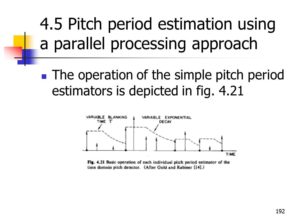
90. 90 3.3 Wave propagation in concatenated lossless tubes Solving we get The quantity is the amount of U k - that is reflected at the junction. The quantity r k is called the reflection coefficient

91. 91 3.3 Wave propagation in concatenated lossless tubes Using the definition of r k we get

92. 92 3.3.3 Relationship to digital filters The form of V a (s) for two tube model: This suggests that lossless tube models have many properties in common with digital filters.

93. 93 3.3.3 Relationship to digital filters To see this, let us consider a system composed of N lossless tubes each of length where, l is the overall length of vocal tract.

94. 94 3.3.3 Relationship to digital filters It is instructive to begin the response of the system to a unit impulse sources The impulse response will be of the form

95. 95 3.3.3 Relationship to digital filters The soonest that an impulse can reach the output is sec. Then successive impulses due to reflections at the junctions reach the output at multiples of seconds later.

96. 96 3.3.3 Relationship to digital filters The system function of such a system will be of the form The factor corresponds to the delay time required to propagate through all N sections.

97. 97 3.3.3 Relationship to digital filters The frequency response is It is easily shown that If the input to the system is band limited to frequencies below,then we can sample the input with period and filter the sampled signal with a digital filter whose impulse response is

98. 98 3.3.3 Relationship to digital filters A typical junction as

99. 99 3.3.3 Relationship to digital filters The difference equation This equation can be written as The term rw + (n) and ru - (n) occur in both equations, 2 out of the 4 multiplications as in fig b.

100. 100 3.3.3 Relationship to digital filters Another representation is This equation requires 1 multiplication and 3 addition. This form of the lossless tube model was first obtained by Itakura and Saito.

101. 101 3.3.4 Transfer function of the lossless tube model Let us seek the transfer function To find V(z), it is most convenient to express U g (z) in terms of U L (z) and then solve for the ratio above.

102. 102 3.3.4 Transfer function of the lossless tube model The z transform equations for this junction are Solving we get

103. 103 3.3.4 Transfer function of the lossless tube model For l=17.5 cm and c=35000 cm/sec, we see 1/2T=Nc/4l=N/2(1000) Hz This implies that there will be about N/2 resonances per 1000 Hz of frequency for a vocal tract of total length 17.5 cm.

104. 104 3.3.4 Transfer function of the lossless tube model

105. 105 3.3.4 Transfer function of the lossless tube model In the above figure, for N=10, 1/T=10 kHz. The largest reflection coefficients occur where the relative change in area is greatest.

106. 106 3.4 Digital Models for Speech Signals Our purpose is to call attention to the basic features of the speech signal and to show how these features are related to the physics of speech production. Sound is generated in 3 ways, and each mode results in a distinctive type of output.

107. 107 3.4 Digital Models for Speech Signals It is simply that a valid approach to representation of speech signals is in terms of a terminal analog model, that is a linear system whose output has the desired speech-like properties when controlled by a set of parameters that are somehow related to the process of speech production.

108. 108 3.4 Digital Models for Speech Signals The model is thus equivalent to the physical model at its terminals but its internal structure does not mimic the physics of speech production. To produce a speech-like signal the model of excitation and the resonance properties of the linear system must change with time.

109. 109 3.4 Digital Models for Speech Signals For many speech sounds, it is reasonable to assume that the general properties of the excitation and vocal tract remain fixed for periods of 10-20 msec. Thus, a terminal analog model involves a slowly time-varying linear system excited by an excitation signal whose basic nature changes from quasi-periodic pulses for voiced speech to random noise for unvoiced cpeesh.

110. 110 3.4 Digital Models for Speech Signals The essential features of the model are depicted in the following fig: Lossless tube model Terminal analog model Lossless tube model Area function U G (n) U L (n) Linear system Parameters U G (n) U L (n)

111. 111 3.4 Digital Models for Speech Signals The relationship between the input and output could be represented by a transfer function V(z) as Where G and α k depends upon the area function.

112. 112 3.4 Digital Models for Speech Signals A complete terminal analog model includes a representation of the changing excitation function and the effects of sound radiation at the lips.

113. 113 3.4.1 Vocal tract The resonances of speech corresponds to the poles of the transfer function V(z). An all pole model is a very good representation of vocal tract effects for a majority of speech sounds; however the acoustic theory tells us that nasals and fricatives require both resonances and anti resonances. In this case, we may include zeros in the transfer function or according to Attal, the effect of a zero to the transfer function can be achieved by including more poles.

114. 114 3.4.1 Vocal tract A typical resonant frequency of the vocal tract is The corresponding complex conjugate poles in the discrete-time representation is

115. 115 3.4.1 Vocal tract The complex natural frequencies of the human vocal tract are all in the left half of the s-plane since it is a stable system.

116. 116 3.4.1 Vocal tract All the corresponding poles of the discrete-time model must be inside the unit circle as required for stability. As long as the areas of the tube model are positive, all the poles of the corresponding V(z) will be inside the unit circle.

117. 117 3.4.2 Radiation If we wish to obtain a model for pressure at the lips, then the effects of radiation must be included. The pressure and volume velocity are related by We desire a similar z-transform relation of the form

118. 118 3.4.2 Radiation Pressure is related to volume velocity by a high-pass filtering operation. At low frequencies it can be argued that the pressure is approximately the derivative of the volume velocity. By using the bilinear transform method of digital filter design it can be shown that a reasonable approximation to the radiation effects is obtained with

119. 119 3.4.2 Radiation The radiation load can be cascaded with the vocal tract model as Vocal tratc model V(z) Parameters U G (n) U L (n) Radiation model P L (n)

120. 120 3.4.3 Excitation The majority of speech sounds can be classed as either voiced or voiceless. We see that in general terms what is required is a source that can produce either a quasi-periodic pulse waveform or a random noise waveform.

121. 121 3.4.3 Excitation A convenient way to represent the generation of the glottal wave is

122. 122 3.4.3 Excitation The impulse train generator produces a sequence of unit impulses which are spaced by the desired fundamental period. Rosenberg in a study of the effect of glottal pulse shape on speech quality, found that the natural glottal pulse waveform could be replaced by a synthetic pulse waveform of the form

123. 123 3.4.3 Excitation

124. 124 3.4.3 Excitation For voiceless sounds the excitation model is much simpler. All that is required is a source of random noise and a gain parameter to control the intensity of the unvoiced excitation. For discrete time models, a random number generator provides a source of flat- spectrum noise.

125. 125 3.4.4 The complete model Putting all the ingredients together we obtain the model

126. 126 3.4.4 The complete model By switching between the voiced and unvoiced excitation generators we can model the changing mode of excitation. The vocal tract can be modeled in a wide variety of ways as we have discussed. In some cases it is convenient to combine the glottal pulse and radiation models into a single system.

127. 127 3.4.4 The complete model In case of linear predictive analysis it is convenient to combine the glottal pulse, radiation and vocal tract components all together and represent them as a single transfer function

128. 128 4 Time domain method of speech processing Our goal in processing the speech signal is to obtain a more convenient or more useful representation of the information carried by the speech signal. The required precision of this representation is dictated by the particular information in the speech signal that is to be preserved or in some case more important.

129. 129 4.1 Time-dependent processing of speech A sequence of samples (8000 samples/sec) representing a typical speech signal is

130. 130 4.1 Time-dependent processing of speech From the figure it is evident that the properties of the speech signal change with time. The underlying assumption in most speech processing schemes is that the properties of the speech signal change relatively slowly with time.

131. 131 4.1 Time-dependent processing of speech This assumption leads to a variety of short-time processing methods in which short segments of the speech signal are isolated and processing as if they were short segments from a sustained sound with fixed propertied.

132. 132 4.1 Time-dependent processing of speech Often these short segments, which are sometimes called analysis frames, overlap one another. The result of the processing on each frame may be either a single number, or a set of numbers. Such processing produces a new time- dependent sequence which can serve as a representation of the speech signal.

133. 133 4.1 Time-dependent processing of speech The speech signal is subjected to a transformation, T, which may be either linear or nonlinear, and which may depend upon some adjustable parameter or set of parameters. The resulting sequence in then multiplied by a window sequence positioned at a time corresponding to sample index n. The product is then summed over all nonzero values.

134. 134 4.1 Time-dependent processing of speech The energy of a discrete time signal is defined as A simple definition of short time energy is That is, the short-time energy at sample n is simply the sum of squares of the N samples n-N+1 through n.

135. 135 4.1 Time-dependent processing of speech In terms of our general expression, the operation T[ ] is simply the square and

136. 136 4.1 Time-dependent processing of speech This figure depicts the computation of the short-time energy sequence.

137. 137 4.1 Time-dependent processing of speech Q n can be interpreted as the output of a linear time-invariant system with impulse response h(n)=w(n) 2. This is shown in the following figure. Linear filter T [ ] Lowpass filter Speech signal QnQn

138. 138 4.1 Short time energy and average magnitude We have observed that the amplitude of the speech signal varies appreciably with time. In particular, the amplitude of unvoiced segments is generally much lower than the amplitude of voiced segments. The short time energy of speech signal provides a convenient representation that reflects these amplitude variations.

139. 139 4.1 Short time energy and average magnitude In general, we can define the short time energy as This expression can be written as

140. 140 4.1 Short time energy and average magnitude The choice of impulse response h(n) or equivalently the window, determines the nature of the short time energy representation. To see how the choice of window affects the short-time energy, we apply h(n) with very long and of constant amplitude. Such a window would be the equivalent of a very narrowband lowpass filter.

141. 141 4.1 Short time energy and average magnitude To effect the window on the time0dependent energy representation can be illustrated by discussing the properties of two representative windows, the rectangular window and the Hamming window

142. 142 4.1 Short time energy and average magnitude The frequency response of a rectangular window is The log magnitude is shown in the following figure.

143. 143 4.1 Short time energy and average magnitude

144. 144 4.1 Short time energy and average magnitude The first zero occurs at analog frequency F=F s /N where F s =1/T is the sampling frequency. This is nominally the cutoff frequency of the lowpass filter corresponding to the rectangular window.

145. 145 4.1 Short time energy and average magnitude Bandwidth of the Hamming window is about twice the bandwidth of a rectangular window of the same length. The Hamming window gives much greater attenuation outside the passband than the comparable rectangular window. The attenuation of both these windows is essentially independent of the window duration. Thus, increasing the length, N, simply decreases the bandwidth.

146. 146 4.1 Short time energy and average magnitude If N is too small, i.e., on the order of a pitch or less, E n will fluctuate very rapidly depending on exact details of the waveform. If N is too large, i.e., on the order of several pitch periods, E n will change very slowly. A suitable practical choice for N is on the order of 100-200 for a 10 kHz sampling rate.

147. 147 4.1 Short time energy and average magnitude

148. 148 4.1 Short time energy and average magnitude The above figure shows the effect of varying the duration of the window on the energy computation. It is seen that as N increases, the energy becomes smoother for both windows.

149. 149 4.1 Short time energy and average magnitude

150. 150 4.1 Short time energy and average magnitude From fig 4.6 and 4.7, the values of E n for the unvoiced segments are significantly smaller than for voiced segments.

151. 151 4.1 Short time energy and average magnitude

152. 152 4.1 Short time energy and average magnitude

153. 153 4.1 Short time energy and average magnitude Fig 4.8 and 4.8 show average magnitude plots corresponding to fig 4.6 and 4.7. For the average magnitude computation, n the unvoiced region, the dynamic range is approximately the square root of the dynamic range for the standard energy computation.

154. 154 4.1 Short time energy and average magnitude Thus the difference in level between voiced and unvoiced regions are not as pronounced as for the short time energy.

155. 155 4.1 Short time energy and average magnitude It is instructive to point out that the window need not be restricted to rectangular or Hamming form, or indeed to any function commonly used as a window in spectrum analysis or digital filter design methods. Furthermore, the filter can be either as FIR or IIR filter.

156. 156 4.1 Short time energy and average magnitude It is not necessary to use a finite length window. It is possible to implement the filter implied by an infinite length window if its z-transform is a rational function. A simple example is a window of the form

157. 157 4.1 Short time energy and average magnitude A value of 0<a<1 gives a window whose effective duration can be adjusted as desired. The corresponding Z transform of the window is from which it is easily seen that the frequency response has the desired lowpass property.

158. 158 4.3 Short time average Zero- Crossing rate In the context of discrete-time signals, a zero crossing is said to occur if successive samples have different algebraic signs. The rate at which zero crossings occur is a simple measure of the frequency content of a signal. A sinusoidal signal of frequency F 0, sampled at a rate F s, has F s / F 0 samples per cycle of the sine wave

159. 159 4.3 Short time average Zero- Crossing rate Each cycle has two zero crossing so that the long-time average rate of zero- crossings is Z=2 F 0 / F s crossings/samples. A definition is

160. 160 4.3 Short time average Zero- Crossing rate The operation is shown in the block diagram. The representation shows that the short-time average zero-crossing rate has the same general properties as the short-time energy and the short time average magnitude.

161. 161 4.3 Short time average Zero- Crossing rate The model of speech production suggests that the energy of voiced speech in concentrated below 3 kHz because of the spectrum fall-off introduced by the glottal wave, where as for unvoiced speech, most of the energy is found at higher frequencies.

162. 162 4.3 Short time average Zero- Crossing rate Since high frequency imply high zero crossing rates, and low frequencies imply low zero crossing rates, there is a strong correlation between zero-crossing rate and energy distribution with frequency. If the zero crossing rate is high, the speech signal is unvoiced, while if the zero-crossing rate is low, the speech signal is voiced.

163. 163 4.3 Short time average Zero- Crossing rate The figure shows a histogram of average zero crossing rates for both voiced and unvoiced speech.

164. 164 4.3 Short time average Zero- Crossing rate The mean short-time average zero crossing rate is 49 per 10 ms for unvoiced and 14 per 10 ms for voiced. Clearly the two distribution overlap so that an unequivocal voiced/unvoiced decision is not possible based on short- time average zero-crossing rate alone.

165. 165 4.3 Short time average Zero- Crossing rate Some examples are

166. 166 4.3 Short time average Zero- Crossing rate The short time average zero crossing rate can be sampled at a very low rate just as in the case of short time energy and average magnitude.

167. 167 4.4 Speech vs. Silence discrimination using energy and zero crossing The problem of locating the beginning and end of a speech utterance in a back-ground of noise is of importance in many areas of speech processing.

168. 168 4.4 Speech vs. Silence discrimination using energy and zero crossing The problem of discriminating speech from background noise is not trivial, except in the case of extremely high signal to noise ratio acoustic environments e.g., high fidelity recordings made in an anechoic chamber or a soundproof room.

169. 169 4.4 Speech vs. Silence discrimination using energy and zero crossing The algorithm to be discussed in this section in based on two simple time- domain measurements- energy and zero crossing rate. Several simple examples will illustrate some difficulties encountered in locating the beginning and end of a speech utterance.

170. 170 4.4 Speech vs. Silence discrimination using energy and zero crossing In the following figure, the background noise is easily distinguished from the speech.

171. 171 4.4 Speech vs. Silence discrimination using energy and zero crossing In this case a radical change in the waveform energy between the background noise and the speech is the cue to the beginning of the utterance.

172. 172 4.4 Speech vs. Silence discrimination using energy and zero crossing In figure 4.14, it is easy to locate the beginning of the speech.

173. 173 4.4 Speech vs. Silence discrimination using energy and zero crossing In figure 4.15, it is extremely difficult to locate the beginning of the speech signal.

174. 174 4.4 Speech vs. Silence discrimination using energy and zero crossing It is very difficult to locate the beginning and end of an utterance if there are: Weak fricatives (f,th,h) at the beginning or end Weak plosive burst (p,t,k) at the beginning or end Nasals at the end Voiced fricatives which become devoiced at the end Trailing off of vowel sounds at the end of an utterance

175. 175 4.4 Speech vs. Silence discrimination using energy and zero crossing In spite of the difficulties posed by the above situations, energy and zero crossing rate representations can be combined to serve as the basis of a useful algorithm for locating the beginning and end of a speech signal.

176. 176 4.4 Speech vs. Silence discrimination using energy and zero crossing One such algorithm was studied by Rabiner and Sambur in the context of an isolated word speech recognition system. In this system a speaker utters a word during a prescribed recording interval, and the entire interval is sampled and stored for processing.

177. 177 4.4 Speech vs. Silence discrimination using energy and zero crossing The algorithm can be described by fig. 4.16

178. 178 4.4 Speech vs. Silence discrimination using energy and zero crossing

179. 179 4.4 Speech vs. Silence discrimination using energy and zero crossing Fig. 4.17 shows examples of how the algorithm works on typical isolated words. The application of zero crossing and average magnitude illustrate the utility of these simple representations in a practical settings. These representations are particularly attractive since very little arithmetic is required for their implementation.

180. 180 4.5 Pitch period estimation using a parallel processing approach Pitch period estimation is one of the most important problems in speech processing. Here we discuss a particular pitch detection scheme first proposed by Gold and later modified by Gold and Rabiner.

181. 181 4.5 Pitch period estimation using a parallel processing approach The reasons for discussing this particular pitch detector are: It has been used successfully in a wide variety of applications It is based on purely time domain processing It can be implemented to operate very quickly on a general purpose compute r It illustrates the use of the basic principle of parallel processing in speech processing.

182. 182 4.5 Pitch period estimation using a parallel processing approach The basic principles of this scheme are as follows: 1. The speech signal is processed so as to create a number of impulse trains which retain the periodicity of the original signal and discard features which are irrelevant to the pitch detection process.

183. 183 4.5 Pitch period estimation using a parallel processing approach 2. This processing permits very simple pitch detectors to be used to estimate the period of each impulse train. 3. The estimates of several of these simple pitch detectors are logically combined to infer the period of the speech waveform.

184. 184 4.5 Pitch period estimation using a parallel processing approach The scheme is

185. 185 4.5 Pitch period estimation using a parallel processing approach The speech waveform is sampled at a rate of 10 kHz. The speech is lowpass filtered with a cutoff of about 900 Hz to produce a relatively smooth waveform. A bandpass filter passing frequencies between 100 Hz and 900 Hz may be necessary to remove 60 Hz noise in some applications.

186. 186 4.5 Pitch period estimation using a parallel processing approach Following the filtering, the “ peaks and valleys” are located and from their locations and amplitudes, several impulse trains are derived from the filtered signal.

187. 187 4.5 Pitch period estimation using a parallel processing approach The 6 case used by Gold and Rabiner are 1. m1(n): An impulse equal to the peak amplitude occurs at the location of each peak. 2. m2(n): An impulse equal to the difference between the peak amplitude and the preceding valley amplitude occurs at each peak.

188. 188 4.5 Pitch period estimation using a parallel processing approach 3. m3(n): An impulse equal to the to the difference between the peak amplitude and the preceding peak amplitude occurs at each peak. 4. m4(n): An impulse equal to the negative of the amplitude at a valley occurs at each valley. 5. m5(n): An impulse equal to the negative of the amplitude at a valley plus the amplitude at the preceding peak occurs at each valley.

189. 189 4.5 Pitch period estimation using a parallel processing approach 6. m6(n): An impulse equal to the negative of the amplitude at a valley plus the amplitude at the preceding local minimum occurs at each valley.

190. 190 4.5 Pitch period estimation using a parallel processing approach

191. 191 4.5 Pitch period estimation using a parallel processing approach

192. 192 4.5 Pitch period estimation using a parallel processing approach The operation of the simple pitch period estimators is depicted in fig. 4.21

193. 193 4.5 Pitch period estimation using a parallel processing approach The performance of the pitch detection scheme is illustrated in fig 4.22

194. 194 4.5 Pitch period estimation using a parallel processing approach The advantage using synthetic speech is that the true pitch periods are known exactly and thus a measure of accuracy of the algorithm can be obtained. The disadvantage of synthetic speech is that it is generated according to a simple model, and therefore may not show any of the unusual properties on natural speech.

195. 195 4.5 Pitch period estimation using a parallel processing approach It has been observed that at the initiation of voicing, the speech is often classified as unvoiced. This result is due to the decision algorithm which requires about 3 pitch periods before a reliable pitch decision can be made-thus a delay of about 2 pitch periods is inherently built into the method

196. 196 4.6 The short time autocorrelation function The autocorrelation function of a discrete tie deterministic signal is defined as If the signal is random or periodic the appropriate definition is If the signal is periodic with period P samples, then it is easily shown that

197. 197 4.6 The short time autocorrelation function Other important properties pf autocorrelation function are It is even function It attains the maximum value at k=0 The quantity Φ(0) is equal to the energy for deterministic signals or the average power for random or periodic signals.

198. 198 4.6 The short time autocorrelation function If we consider properties 1 and 2, for the periodic signals the autocorrelation function attains a maximum value at samples That is regardless of the time origin of the signal, the period can be estimated by finding the location of the first maximum in the autocorrelation function

199. 199 4.6 The short time autocorrelation function The short time autocorrelation function is defined as The equation can be interpreted as: First a segment of speech is selected by multiplication by the window, then the deterministic autocorrelation definition is applied to the window segmented of speech. It is verified that

200. 200 4.6 The short time autocorrelation function First note that If we define Then the equation comes as

201. 201 4.6 The short time autocorrelation function Thus the value at time n of the kth autocorrelation lag is obtained by filtering the sequence x(n)x(n-k) with a filter with a impulse response h k (n).

202. 202 4.6 The short time autocorrelation function The computation of the short time autocorrelation function is usually carried out by using the following equation

203. 203 4.6 The short time autocorrelation function If the window w’ is of finite duration then the above equation comes as

204. 204 4.6 The short time autocorrelation function

205. 205 4.6 The short time autocorrelation function

206. 206 4.6 The short time autocorrelation function By comparing the above figures it can be seen that the rectangular window gives a much stronger indication of periodicity than the Hamming window.

207. 207 4.6 The short time autocorrelation function An important issue is how N should be chosen to give a good indication of periodicity. Conflicting requirement: Because of the changing properties of speech signal, N should be small. It should be clear that to get any indication of periodicity in the autocorrelation function, the window must have a duration of at least two periods of the waveform.

208. 208 4.6 The short time autocorrelation function The dotted lines are plots pf the equation

209. 209 4.6 The short time autocorrelation function The modified short time autocorrelation function is defined as This expression can be written as

210. 210 4.6 The short time autocorrelation function

211. 211 4.6 The short time autocorrelation function Where We can choose the window w2 to include samples outside the nonzero interval of window w1. That is

212. 212 4.6 The short time autocorrelation function Thus the equation can be written as This is the modified short time autocorrelation function. It has the properties of a cross correlation function, not an autocorrelation function.

213. 213 4.6 The short time autocorrelation function

214. 214 4.6 The short time autocorrelation function

215. 215 4.7 The short average magnitude difference function A technique that eliminates the need for multiplications is based upon the idea that for a truly periodic input of period P, the sequence would be zero for For short segments of voiced speech it is reasonable to expect that d(n) will be small at multiples of the period, but not identically zero.

216. 216 4.7 The short average magnitude difference function The short time average magnitude difference function is defined as If x(n) is close to being periodic in the interval spanned by the window, then γ n (k) should dip sharply for k=P,2P…

217. 217 4.7 The short average magnitude difference function It can be shown that It is reported that β(k) varies between 0.6 and 1.0 with different segments of speech, but does not change rapidly with k for a particular speech segment.

218. 218 4.7 The short average magnitude difference function

219. 219 4.7 The short average magnitude difference function The AMDF function is implemented with subtraction, addition and absolute value operations, in contrast to addition and multiplication operations for autocorrelation function.

220. 220 4.8 Pitch Period Estimation using the Autocorrelation Function A technique called center clipping can be used for spectrum flattening. The center clipped speech signal is obtained by a nonlinear transformation y(n)=C[x(n)]

221. 221 4.8 Pitch Period Estimation using the Autocorrelation Function

222. 222 4.8 Pitch Period Estimation using the Autocorrelation Function Here the peaks are converted to pulses consisting of the part of each peak that exceeds the clipping level.

223. 223 4.8 Pitch Period Estimation using the Autocorrelation Function

224. 224 4.8 Pitch Period Estimation using the Autocorrelation Function For high clipping levels, fewer peaks will exceed the clipping level and thus fewer pulses will appear in the output, and therefore, fewer extraneous peaks will appear in the autocorrelation function.

225. 225 4.8 Pitch Period Estimation using the Autocorrelation Function

226. 226 4.8 Pitch Period Estimation using the Autocorrelation Function As the clipping level is decreased, more peaks pass through the clipper and thus the autocorrelation function becomes more complex. The implication of this example is that the clearest indication of periodicity is obtained for the highest possible clipping level.

227. 227 4.8 Pitch Period Estimation using the Autocorrelation Function It is possible that the amplitude of the signal may vary appreciably across the duration of the speech segment so that if the clipping level is set at a high percentage of the maximum amplitude across the whole segment, there is a possibility that much of the waveform will fall below the clipping level and be lost. For this reason, Sondhi’s original proposal was to set the clipping level at 30% of the maximum amplitude.

228. 228 4.8 Pitch Period Estimation using the Autocorrelation Function A procedure which permits a greater percentage (60-80%) to be used it to find the peak amplitude in both the first third and last third of the segment and set the clipping level at a fixed percentage of the minimum of these two maximum levels.

229. 229 4.8 Pitch Period Estimation using the Autocorrelation Function A simple modification of the center clipping leads to a great simplification in computation of the autocorrelation function with essentially no degradation in utility for pitch detection.

230. 230 4.8 Pitch Period Estimation using the Autocorrelation Function The computation of the autocorrelation function for a 3-level center clipped signal is particularly simple. The autocorrelation function is

231. 231 4.8 Pitch Period Estimation using the Autocorrelation Function The above function can have only three different values

232. 232

233. 233 4.8 Pitch Period Estimation using the Autocorrelation Function The scattering of points that are obviously errors due to the fact that a peak at a short lag was greater than the peak at the pitch period. The pitch period averages between 100 and 150 samples so that the inherent fall-off of the autocorrelation function causes significant attenuation of the peak at the pitch period.

234. 234 4.8 Pitch Period Estimation using the Autocorrelation Function Most of the errors have been eliminated by the inclusion of clipping and furthermore there is no significant difference between the two result. A few obvious errors remain in both pitch contours. These errors can be effectively removed by a nonlinear smoothing method to be used.

235. 235 Chapter 7 Homomorphic Speech Processing

236. 236 7.0 Introduction Since the excitation and impulse response of a linear time-invariant system are combined in a convolutional manner, the problem of speech analysis can also be viewed as a problem in separating the components of a convolution. In this chapter, after giving a brief introduction to the general theory of homomorphic systems for convolution, we shall discuss a variety of applications of homomorphic deconvolution in the analysis of speech signals.

237. 237 7.1 Homomorphic systems for convolution Homomorphic systems for convolution obey a generalized principle of superposition.

238. 238 7.1 Homomorphic systems for convolution

239. 239 7.1 Homomorphic systems for convolution For convolution linear time invariant system can be expressed as We define a class of system having the superposition law where addition is replaced by convolution.

240. 240 7.1 Homomorphic systems for convolution

241. 241 7.1 Homomorphic systems for convolution Any homomorphic system can be represented as a cascade of three homomorphic systems as

242. 242 7.1 Homomorphic systems for convolution

243. 243 7.1 Homomorphic systems for convolution The inverse characteristics is defined as

244. 244 7.1 Homomorphic systems for convolution The mathematical representation is After taking Z transform

245. 245 7.1 Homomorphic systems for convolution Homomorphic deconvolution

246. 246 7.1 Homomorphic systems for convolution The inverse homomorphic system

247. 247 7.1 Homomorphic systems for convolution Here, uniqueness of the response of log of a complex variable should be considered. As long as we are in unit circle, it is possible.

248. 248 7.1 Homomorphic systems for convolution So the output homomorphic system for deconvolution can be obtained by inverse Fourier Transform: We call this output as complex cepstrum.

249. 249 7.1 Homomorphic systems for convolution Complex cepstrum is inverse F. T. of logarithm of the spectrum of a signal. Without considering the imaginary part, we have real cepstrum

250. 250 7.1.1 the properties of Complex Cepstrum If they have rational z-transform

251. 251 7.1.1 the properties of Complex Cepstrum If we are on unit circle has only imaginary part. By using expansion we get

252. 252 7.1.1 the properties of Complex Cepstrum We observe that in general the complex cepstrum is nonzero and of infinite extent for both positive and negative n, even though x(n) may be causal, stable and even of finite duration.

253. 253 7.1.1 the properties of Complex Cepstrum Furthermore, it is apparent that the complex cepstrum is a decaying sequence which is bounded by

254. 254 7.1.1 the properties of Complex Cepstrum For Such signal are called minimum phase signal.

255. 255 7.1.1 the properties of Complex Cepstrum So the cepstrum is obtained by taking only real part of F. T. But, since the real part of F. T. is the F. T. of the even part of signal, then:

256. 256 7.1.1 the properties of Complex Cepstrum It can be shown

257. 257 7.1.1 the properties of Complex Cepstrum For minimum phase signal, we can proof that:

258. 258 7.1.1 the properties of Complex Cepstrum Similar results can be obtained in the case when no poles or zero inside the circle. Such signals are called maximum phase signal.

259. 259 7.1.1 the properties of Complex Cepstrum The recursion formula for the complex cepstrum is:

260. 260 7.1.1 the properties of Complex Cepstrum One important example is for simple pulse shape signal. The z-transform

261. 261 7.1.1 the properties of Complex Cepstrum

262. 262 7.1.1 the properties of Complex Cepstrum The fact that the cepstrums appear at the same pulses position as like as original signal, is very important for speech and echo analysis.

263. 263 7.1.2 Computational considerations For z-transform, we can use DFT, if we are on unit circle and then using FFT, instead of DFT.

264. 264 7.1.2 Computational considerations For cepstrum

265. 265 7.1.2 Computational considerations

266. 266 7.2 The complex cepstrum of speech We can combine the homomorphic filtering theory with the model of speech signal, previously obtained, to get a useful application.

267. 267 7.2 The complex cepstrum of speech For voice sound, the linear system combined by 1-Glotis wave G(z) 2-Vocal cavity filter V(z) 3-Radiation from lips R(z)

268. 268 7.2 The complex cepstrum of speech The general model The radiation effect Thus

269. 269 7.2 The complex cepstrum of speech For voice we have So, we have only poles inside unit circle. For unvoice and nostril voice, we have both ploes and zeros. Zeros could be inside and outside unit circle. But all poles are located inside unit circle. However, since v(n) is real, all poles & zeros are in the shape of complex conjugate.

270. 270 7.2 The complex cepstrum of speech For radiation from lips, R(z), we use more emphasis at high frequencies. For voice, the glottal pulses have finite duration pulses and they appear as zeros inside or outside of unit circle.

271. 271 7.2 The complex cepstrum of speech For voice, combination of G(z), V(z), R(z) generally in “non minimum phase” signal, then, we should have both positive and negative time non-zeros complex cepstrum coefficients.

272. 272 7.2 The complex cepstrum of speech According to previously obtained equations, for computing the complex cepstrum coefficients, it is resulted that these coefficients are rapidly decayed by time (n).

273. 273 7.2 The complex cepstrum of speech Another important point is that these coefficients are appeared in multiply integer for period of the periodic pulses. Therefore, it is expected that for voice, these coefficients will be appeared in multiply of original signal period (pitch period).

274. 274 7.2 The complex cepstrum of speech

275. 275 7.2 The complex cepstrum of speech

276. 276 7.2 The complex cepstrum of speech a) Original signal is multiplied by a Hamming window. b) is log of DFT, the periodicity in this figure is due to periodic signal and it is similar to formant. c) is phase of DFT d) is unwarapped continuous phase

277. 277 7.2 The complex cepstrum of speech e) is complex cepstrum. We can notice the peaks at both positive and negative time, which are corresponding to pitch period. They are decayed by time rapidly. Cepstrum is inverse of Fourier Transform of logarithm of Fourier Transform magnitude (putting phase to zero). So, it is important for speech analysis.

278. 278 7.2 The complex cepstrum of speech At first we insert the speech signal s(n) and multiply by window w(n), then we calculate the cepstrum. The desired component of cepstrums are separated by a “cepsrtum window l(n)”. Then, the resultant windowed complex cepsrtum are inserted into inverse system for deconvolution.

279. 279 7.2 The complex cepstrum of speech If (for low time window) In fig. 10, after smoothing window w(n), l(n) the resulting cepstrum shown in fig 10(c). This is an approximation of impulse response of vocal cavity.

280. 280 7.2 The complex cepstrum of speech

281. 281 7.2 The complex cepstrum of speech

282. 282 7.2 The complex cepstrum of speech

283. 283 7.2 The complex cepstrum of speech If (for high time window) In fig 10(d,e,f), will be obtained for log DFT and phase & high time cepstrum components. These are similar to series of pulses representing an estimation of excitation p(n).

284. 284 7.2 The complex cepstrum of speech For an unvoiced speech, fig 11,

285. 285 7.2 The complex cepstrum of speech

286. 286 7.2 The complex cepstrum of speech Comparing fir 7.8 and 7.11(c), we can see that cepstrum is a suitable approach for voice unvoice detection. Pitch can be obtained in voice by high time window in cepstrum. Formant frequency can be obtained in log |DFT| of low time window cepstrum..

287. 287 7.3 Pitch detection There is a peak in the cepstrum at the fundamental period of the input speech segment. No such peak appears for the unvoiced speech segment. These properties can be used as a basis for determining whether a speech segment is voiced or unvoiced.

288. 288 7.3 Pitch detection If cepstrum peak is above a pre-set threshold, the input speech segment is likely to be voiced and the position of the peak is a good estimate of the pitch period. If the peak does not exceed the threshold, the input speech is unvoiced.

289. 289 7.3 Pitch detection

290. 290 7.3 Pitch detection

291. 291 7.3 Pitch detection Typically the cepstrum is computed once every 10-20 msec since the excitation parameters do not change rapidly in normal speech.

292. 292 7.3 Pitch detection From fig. 7.12, the first seven 40 msec intervals corresponds to unvoiced speech, while the remaining cepstra indicate that the pitch period increases with time.

293. 293 7.3 Pitch detection The signal can deviate from the model if it is extremely bandlimited. In this case there is only one peak in the log spectrum. If there is no periodic oscillation in the log spectrum, there will be no peak in the cepstrum. For the shortest pitch periods, the pitch peak occurs is a region where the other cepstrum components have died out appreciably.

294. 294 7.3 Pitch detection With appropriate window length at input, the location and amplitude of the cepstrum peak provide a reliable pitch and voicing estimate most of the time. Where cepstrum fails to clearly display the pitch and voicing, the reliability can be improved by the addition of other information such as zero crossing rate and energy and by forcing the pitch and voicing estimates to vary smoothly.

295. 295 7.3 Pitch detection

296. 296 7.3 Pitch detection