1. The Computational Nature of Language Learning and Evolution 10. Variations and Case Studies Summarized by In-Hee Lee 2009. 08. 25.

2. Chapter Overview 001 Population at t … 1 L1L2 L1 Child Population … Population at t + 1 … P1P1 P2P2 Sampled sentences are presented 0110 Infinite Population Size? Shared Sentence Distribution? Monolingual Learning?

3. 10.1 Finite Populations Infinite population  Deterministic dynamic systems on the population evolution Finite population  Stochastic dynamic systems on the population evolution For large population size, the two dynamic systems behave similarly. For small population size, the two differ substantially.

4. 10.1 Finite Populations Two language system (infinite population)   t : the proportion of L 1 speakers in generation t.  f : the probability a typical child acquires L 1 (following A) on taking k examples. Finite population size N  The linguistic configuration of the population in generation t  The average linguistic behavior of the population  For very large N, The fraction of L 1 speakers is close to the infinite population case. 1: the ith adult in generation t speaks L 1

5. 10.1 Finite Populations The evolution of Y(t) over time can be characterized by a Markov chain with N + 1 states {0/N, 1/N, …, N/N}.  All children use the same learning algorithm A. 011 X i (t+1) … L2L2 L1L1 L1L1

6. 10.1 Finite Populations Evolutionary behaviors as a function of N  Large N The finite population case shows dynamic behavior that is a noisy version of finite population case’s where the variance of the noise is bounded by 1/4N. (proof)proof The larger N is, the more closely the dynamics will resemble the behavior of the infinite system.  Small N The stationary distribution of the Markov chain characterize how often the population is in the state Y(t) = i / N (proportional to the probability that Y(t) = (i–1)/N). Behavior at small N may be qualitatively different from the behavior at large N.  Peak inversion of TLA learner  Cue learner with finite k.

7. 10.1 Finite Populations  Example of TLA learner

8. 10.1 Finite Populations TLA learner N = 150 N=75 N=30

9. 10.1 Finite Populations : Different Behaviors TLA learner Cue learner  The infinite population shows a bifurcation  The finite population always converge eventually to 0 (all L2 speakers).  The chain will eventually settle to 0. N=25 N=23 T 0j ==0

10. 10.1 Finite Populations Summary  If there are no extremal fixed points (neither 0 nor 1 is a fixed point), the behavior of the finite population is similar to the infinite one for large N and may differ for small N.  Extremal fixed points correspond to absorbing states of the finite population. General question reduces to understanding the relation between the deterministic dynamical system (infinite population) and the corresponding stochastic process (finite population).

11. 10.2 Spatial Effects So far, we have assumed all children receive their primary linguistic data from the same source distribution  All children are exposed to the same linguistic environment.  A “perfectly mixed” social-connectivity pattern. More realistic assumption  Children born in different neighborhoods are exposed to different source distributions, having different linguistic experiences. Assume the geographic extent of population as the unit square.  The linguistic distribution of the population in space and time Proportion of L 1 users at location (x, y) and time t.

12. 10.2 Spatial Effects The probability a child at location (x, y) would acquire L 1 using a learning algorithm A with k examples.  The dynamics depends on the characteristics of f. Simple example where f has two stable fixed points. In the basin of one attractor. In the basin of the other attractor. In the basin of one stable state. In the basin of the same attractor.

13. 10.2 Spatial Effects Influence function  I(z,x) : the influence of speakers at location x on learners at location z. For a learner at location z,  The overall probability with which the learner encounter a speaker of L 1 at time t  Then the evolution of language is characterized by

14. 10.2 Spatial Effects Three propositions for monotonic f with two stable attractors and an unstable fixed point (proofs).proofs 1.If gt is the constant function, it remains so for all time. The evolution of the constant is characterized by f. If there is no spatial diversity to begin with, such diversity will not arise. 2.If at all locations z, we have gt > (attractor threshold), then spatial diversity will be eliminated. Even if there is diversity to begin with, if all the initial conditions lie in the basin of one attractor, the spatial diversity will eventually be eliminated as the linguistic composition moves toward that attractor. 3.Even though f has no cycles, the spatial evolution could display oscillations because of spatial interactions. The spatial distribution of language and the interactions between different regions may have considerable effect on the dynamics.

15. 10.3 Multilingual Learners Multilingual acquisition  Whether and when the learning child becomes bilingual?  How the learning child know that there are multiple different linguistic systems in its environment?  One approach – categorize the individuals into linguistic groups and acquire different systems from the groups. Useful when different languages use different lexical items. What if the linguistic systems interact?  If they share lexical items but have different grammatical rules?  Child acquires a mixture of competing systems that it uses simultaneously. Linguistic knowledge as a distribution over competing grammatical systems.

16. 10.3 Multilingual Learners Bilingual model as a lambda learner  Individuals are bilingual with two internal grammars (g1 and g2).  Each adult has its own characteristic (frequency of usage between grammars).  Source sentence distribution for a child (proof)proof  Children use the same learning algorithm with finite primary linguistic data to estimate its own.  Three candidate algorithms L1L2 n1n2n3

17. 10.3 Multilingual Learners  Evolutionary consequences according to different learning algorithms (proof)proof  Different -estimation algorithms lead to different dynamical systems.  Three dynamical systems have different evolutionary consequences. A1A1 A2A2 A3A3 u t => 0 (for all a > 0)u t => 1 (for all b > 0)

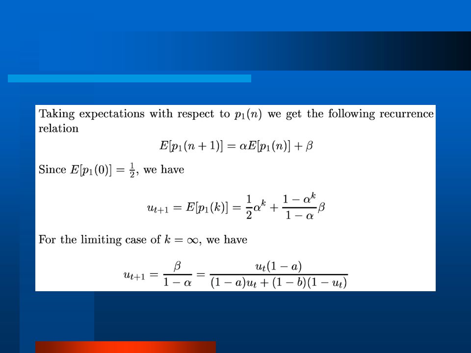
18. 10.3 Multilingual Learners Bilingual model as memoryless online learner  p i (t) : the weight on grammar i upon seeing t sentences.  Assume uniform initial prior (p 1 (0) = p 2 (0) = 0.5).  Memoryless online learning algorithm  Evolutionary consequence is the same as the case of A 1. (proof)proof

19. 10.3 Multilingual Learners Differences between bilingual and monolingual learning when batch-learning algorithms are used.  Monolingual learning: two stable equilibria (homogeneous population using L1 speakers or L2 speakers). No gradual transition between two stable populations.  Bilingual learning: one stable equilibrium with two fixed points. Switch in usage frequencies a, b would cause a switch in the stability of the population.

20. 10.4 Conclusions The finiteness of population size  For large, medium population sizes, the stochastic behavior is like a noisy version of the deterministic dynamics of infinite population.  For small population sizes, the behavior can be systematically different. The effects of spatial organization of the population  Dialects can be formed depending upon the initial conditions of the population in that region. The population dynamics for multilingual learners  Two different bilingual learning procedures and their dynamical behaviors.

21. Proof for Finite Populations Evolutionary behavior as a function of N  Large N : by central limit theorem,  Since,  The finite population case shows dynamic behavior that is a noisy version of finite population case’s where the variance of the noise is bounded by 1/4N.  The larger N is, the more closely the dynamics will resemble the behavior of the infinite system. <= Same as the infinite population case

22. Proofs for Spatial Effects Proposition 10.1 Proposition 10.2

23. Proofs for Spatial Effects Proposition 10.3

24. Proofs for Multilingual Learners Bilingual individual and the population  The probability with which an adult produce a sentence P i (s) : the probability that s is generated using grammar g i.  The total probability distribution over sentences

25. Proofs for Multilingual Learners

26. Dynamics of memoryless bilingual online learner