1. Lecture 3 3.1Supply-side structures, policies and shocks 3.2 Price push factors (z p ) on PS curve [W/P=λ.f(μ,z p )] 3.3Wage push factors (z w )on WS curve [W/P=b(λ,E,z w )] 3.4 Unions, wage-setting and the ERU 3.5 Hysteresis – how actual U affects ERU 3.6 Conclusions from Chapter 3.7 Ball and Mankiw’s analysis of supply-side factors shifting the natural rate of unemployment (US 1960-90’s)

2. 3.1Supply-side structures, policies and shocks Supply-side policies refer to those that shift the wage-setting (WS) and price-setting (PS) curves – WS shifted by changes in unemployment benefits, minimum wages, employment legislation, child-care policy – PS shifted by – changes in taxes or competition policies Note: Taxes and govt spending affect both the demand and supply, but in this lecture we are focusing on the supply-side effects of these policies Supply-side changes in WS and PS effect the level of equilibrium output ye and thereby effect the equilibrium rate of unemployment ERU (aka the Nairu)

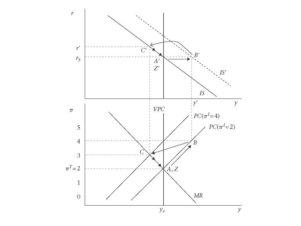
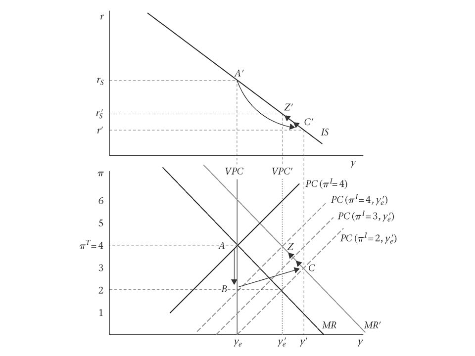
3. Effect of a supply-side shock that reduces union bargaining power In Fig 4.1 a downward shift in WS leads to a shift form A’ to Z’ i.e. employment increases from Ee to E’e at an unchanged real wage Scenario 1 (if there are lags in the CB’s response to the shift in WS): – then the CB will take some time to realise that there are disinflationary pressures in the economy and the CB will only reduce the interest rate once the lower inflation rate form 4% to 2% has revealed itself i.e. the move from A to B, – in the labour market there is downward pressure on wages as more people are willing to work at the going wage and at a given level of employment there is downward pressure on wages (e.g. at B’) – then the CB lowers the interest rate and stimulate AD moving economy from B to C – Due to the lagged response the r overshoots from r s to r’ before moving to r’ s ) Scenario 2 (if CB correctly anticipates the shift in WS): – then the CB will realise that there will be disinflation in the economy and will also realise that equilibrium employment has shifted to E’e and equilibrium output to y’e – The CB will immediately in the first period cut the interest rate form r s to r’ s (with no overshooting) – The economy would move straight from A to Z and inflation will always remain on target (π T ) – in the labour market there is no downward pressure on wages as the cut in the interest rate means that there is increased demand for along with increased supply of labour

5. Comparing demand and supply shocks Note: Supply shocks differs from demand shocks as follows: For a supply shock: – to a new equilibrium output (y’e) level – the MR schedule to point at which inflation target (π T ) intersects new equilibrium output (y’e) For a demand shock: – The equilibrium output (y’e) level and the MR schedule do NOT SHIFT

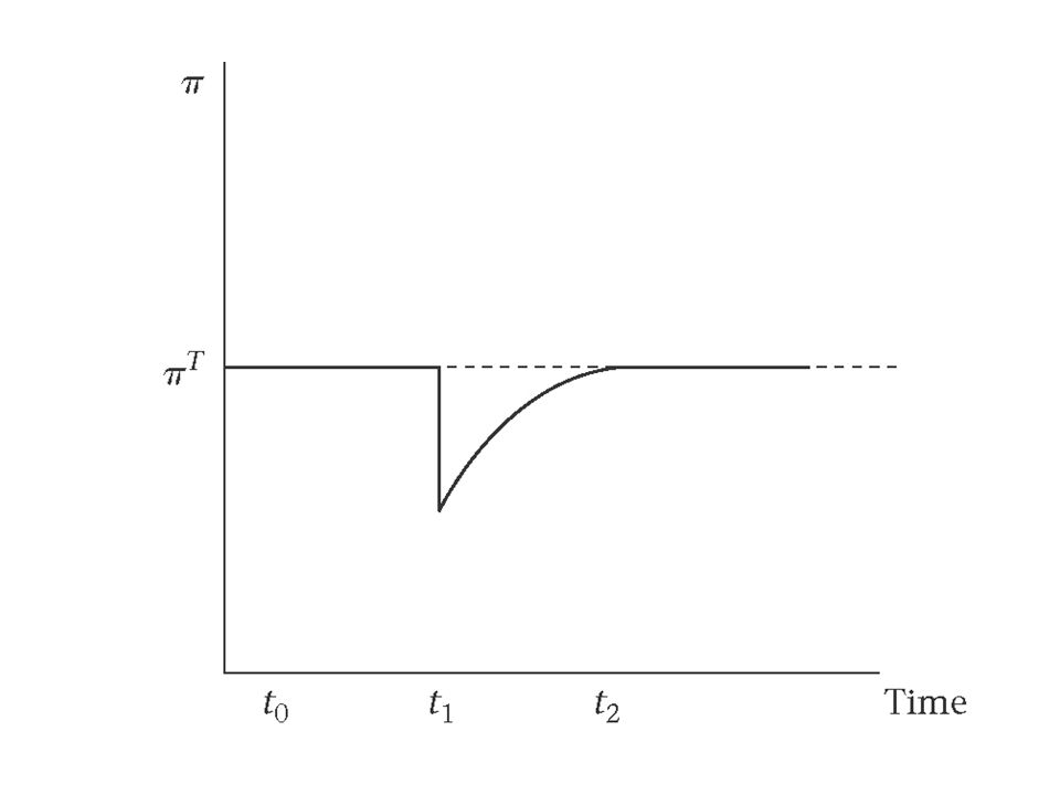
7. Time profile of inflation Scenario 1 (if there are lags in the CB’s response to the shift in WS): – the time profile of inflation is given by Fig 4.2 – inflation falls sharply and then returns to (π T ) Scenario 2 (if CB correctly anticipates the shift in WS): – Inflation remains constant at (π T )

9. IS curve and MR curve (where CB response is sluggish) IS CURVE Initially and temporarily the CB overshoots as it sets r to r’ as the sluggish CB must re-inflate the system due to wages and prices falling and to achieve π T (in the IS diagram 4.3 there is a cut in the interest rate from r s to r’) (from A’ to C’) Overall (the move is from r s to r’ s ) (from A’ to Z’) - the stabilising interest rate r s ’ is lower in the new equilibrium because equilibrium output is higher due to the supply-side shift (AS  ) and a lower real interest rate is required to provide the appropriate level of AD (AD  ) MR CURVE MR shifts from MR to MR’ – comprising the new objective point due to the fall in wages at (π T, y’e) (point Z) and the subjective preferences of the CB’s loss function (giving the slope of the MR curve) Once the economy is on the new MR line MR’ the adjustment takes place from C’ to Z’ (i.e. r remains below r’s but rises towards r’s as inflation rises to π T )

11. 3.2 Price push factors PS – price-push factors (z p ) shift the PS curve And cause supply-side shifts in equilibrium output ye and the equilibrium rate of unemployment PS is given by W/P=λ(1 – μ) – PS shifts up with productivity λ gains (increasing equilibrium output ye and employment), and – PS shifts down with increases in mark-up/pricing power μ, (decreasing equilibrium output ye and employment) If we include the price push effects of taxes (called the ‘tax wedge’) then: – PS is given by W/P = λ(1 – μ) / (1+t d )(1 + t v ) or – W/P=λ.f(μ,z p ), where: PS shifts up with increased productivity λ PS shifts down with increased pricing power μ, and PS shifts down with increased price-push factors (z p ) such as direct taxes t d and indirect taxes t v

12. Note on the tax wedge Relevant to WORKER utility: – w = W/P c is the real consumption wage, where – W = the post-tax money wage, and – P or P c = the consumer price index (inclusive of indirect taxes) (ie P c = P(1+t v )) Relevant to FIRM utility: – w = W / P – W is the full cost to company real product wage (inclusive of taxes and non- wage labour costs), and – P the price that the firm gets for its product (excluding indirect taxes) The difference between the real consumption wage and the real product wage is the Tax Wedge The tax wedge shows up as a price-push factor (z p ) and any rise in taxes or the tax wedge pushes the PS curve down Any increase in direct or indirect taxes increases the tax wedge, eg raises VAT, raise tax on employees salaries, raises the cost of employment, etc. The increase in taxes shifts PS downwards, reducing equilibrium output and employment

13. Change in taxes shift PS curve Any fall in taxes implies an upward shift in the PS curve (as t d and t v are in the denominator) of PS equation i.e. the real wage is higher if the tax take is smaller => WS and PS curves intersect at a higher level of employment Conclusion: higher taxes (indirect and direct taxes) mean a larger tax wedge which will result in higher unemployment (lower real wage and PS curve shifts downwards)

14. Price-push factors (including tax wedge) PS curve can be written compactly as: W/Pc = λ.f(μ, z p ) PS curve shifts up (employment up, equilibrium output up and real wage up) where: – The is a rise in productivity (λ) – Fall in the mark-up price μ (increased competition) – There is a fall in the tax wedge (z p ) z p is set of price-push variables including – the tax wedge, business registration costs, employment regulations (“lower the cost of doing business”) – Although the cost of health and safety regulations (z p ) may be off-set by the compensating positive effect on productivity (λ) – High real interest rates are clearly a demand side instrument, but they also have supply-side effects and can be included as a price-push factor (z p ) (known as the “cost channel”). They also could be viewed as reducing productivity (λ) (due to cost of capital) and resulting in higher mark-up (μ) as firms attempt to cover borrowing costs.

15. 3.3Wage-push factors WS equation can be written as: W/P =b (E,z W ) z W are wage-push variables including institutional, policy, structural and shock variables WS shifts down (increasing employment levels as z W falls) where: – There is a fall in employment benefits (or ratio of benefits to average wage) – Union protection falls or unions weaker (reducing gap between WS and labour supply curve) – Unions / employees exercise bargaining restraint e.g. a wage accord (e.g. proposal for wage accord for high and low income earners in South Africa’s New Growth Path - 2010)

16. Wage-push factors and productivity increases There is debate as to how to include labour productivity changes (λ) in the WS and PS equations First approach - λ is included in WS and PS symmetrically (ie WS rise is equal to the PS rise as a result of λ) => no change in ERU (this is supported by stylised fact that productivity has been rising but the ERU has not changed), in this approach wage aspirations rise inline with productivity – Specified as W/P= λ b(E,Zw) (full symmetrical effect of λ is assumed) Second approach – λ changes take some time to for the change in productivity trend to influence wage-setting behaviour (slow adjustment or lag so PS and WS do not shift symmetrically) => a slow down in λ will lead to a rise in ERU and a increase in λ will lead to a fall in ERU (See Ball and Mankiw (2002) on productivity and the Nairu) (Reading pack 2) – Specified as W/P = b(λ,E,Zw) (λ is inside b function to reflect uncertainty of the adjustment)

17. Wage-push factors and training programmes Training may have two effects: First – training increases productivity of work force and pushes PS upwards (and possibly WS curve up symmetrically or lagged) increasing wages and employment Second – education may weaken the bargaining power of employees shifting the WS curve downwards (increasing employment but decreasing wages) Both effects are theoretically possible and the result will depend on the specific empirical circumstances e.g. in SA would widening the skills pool assist in reducing the premium on skills and thus narrow the wage gap?

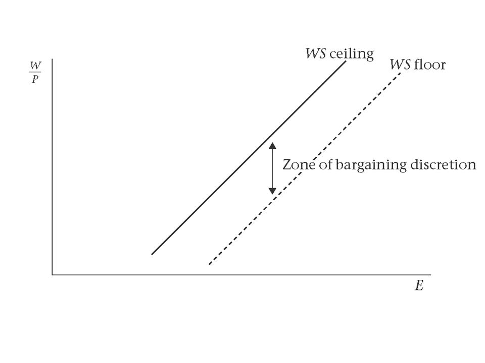
18. Wage-push factors and wage accords Wage accord or incomes policy agreements can be entered into between labour, business and government which have the effect of limiting wage increases and lowering the WS curve See Fig 4.4 where it is assumed that wage negotiations outcomes can results in setting wages between two limits – the WS ceiling set by employers (they will not go higher) and the WS floor set by employees (they will not go lower) The gap between the ceiling and the floor is termed the “zone of bargaining discretion”

20. Wage-push factors and wage accords (cont.) Question why don’t unions always insist on the WS ceiling? Because of unions concern for long-run future of the industry, maximum industrial action may jeopardise investment plans in the industry (unions and employers are in a relationship that is simultaneously antagonistic and co- dependent) Where there is a wage accord (or incomes policy) the WS curve moves downwards in the zone of bargaining discretion (often with govt offering policy measure supported by the unions e.g. tax cuts / pension policy, etc.) Examples of successful wage accords are Netherlands (1982) and Ireland (1987) where there was wage restraint and increased employment assisted by the productivity growth of the 1990’s (In SA despite wage accord proposals – relations have been relatively conflictual and antagonistic in the post 1994 period)

21. Notes on Australian Labour Accord in the 1980’s There was a 1983 accord between the Australian Labour Party (ALP) and the Australian Council of Trade Unions (ACTU), which served as a platform to bring the labour party to power and secure long-term gains for the broader working class in Australia. In 1983 the Australian economy was suffering stagflation (stagnant employment growth and inflation) and on the eve of elections, which Bob Hawke’s Australian Labour Party eventually won, the ALP and ACTU signed an accord which sought to secure employment growth, put in place tax cuts for the poor as well as increased social security, parental rights of workers and social services aimed at benefiting poor families. Through a process of negotiation the ALP and ACTU arrived at a common “realistic appraisal of the economic situation” and “identified jointly how best long term gains could be made for the working class”. The working class, which he defined as comprising three components, that is, the organised working class, the unorganised working class and the unemployed.

22. Australian Labour Accord (cont). The following gains were achieved: – thirteen years of wages increases, although moderate, were better than would have been secured without the accord, – a record number of jobs were created and stagflation was ended, – the working week was shortened and parental rights were secured, – the economy was made more competitive and was opened up to international trade in a sustainable way, – a superannuation savings and pension scheme was created, and – a free health care systems was put into place. Looking beyond the immediate interests of current union membership, goals such as employment creation, social security gains and international competitiveness were seen as important objectives by the ALP and ACTU. “Simple wage gains can be quickly eroded by inflation, but institutional changes have the potential to benefit workers forever” – claimed the ACTU.

23. Analysis of why wage accord is difficult for unions If there are many unions competing in the economy then there is an incentive for unions to defect from the wage accord and try and secure higher wages Game theory’s Prisoner Dilemma framework is useful to understand this incentive to defect / confess: – If one confesses and the other does not he gets 0 years and the other gets 20 years – If both confess they both get 10 years – If neither confess they both get 2 years – The dominant strategy is to confess (get 0 years for one and 20 for the other or 10 years each) even though combined utility is maximised if neither confess (2 x 2yrs in jail) – 0 + 20 or 10 + 10 > 2 + 2 i.e. loss is minimised at 2 + 2 but prisoner’s cannot co-ordinate their decision for the optimal outcome

24. Unions incentive to defect as prisoners dilemma Game theory’s Prisoner Dilemma framework is useful to understand this incentive to defect from the wage accord: – If one union defects from wage accord and the other does not the defecting union gets higher wages (and reduced employment) – If both unions defect they both get higher wages (but reduced employment) – If neither unions defects they both get lower wages but increased employment (which is the best social outcome) – The dominant strategy is to defect with the result of higher wages and lower employment even though the best employment outcome is for no defection For this reason the wage accord is more possible/more likely in economies where there are fewer competing unions and where there is a recognised dominant union leading highly centralised bargaining (the co-ordination problem is easier to resolve optimally)

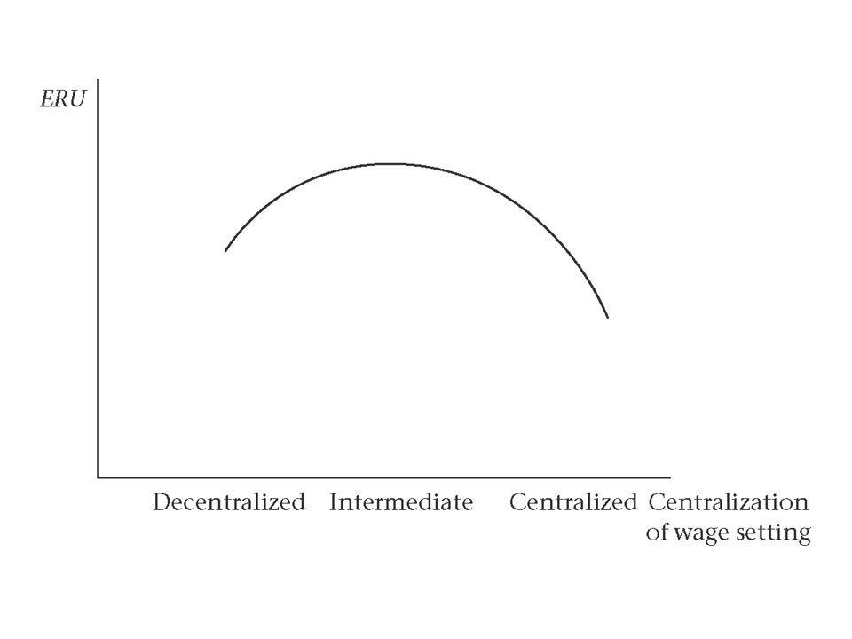
25. 3.4 Unions, wage-setting and the ERU Calmfors and Driffill (1988) posited a humped-shaped relationship between the degree of centralisation of wage setting and the ERU (see Fig 4.7) A low ERU is consistent with highly decentralised or highly centralised wage bargaining. In between is the intermediate degree of centralisation (where there may be strong competition between unions undermining wage accords) where the ERU is higher. (Post 94 SA is probably best characterised as being in this zone of intermediate centralisation – not only due to union competition but also policy and political contestation) An implication of Calmfors and Driffill’s thesis is that union strength is not necessarily associated with an upward push in the WS curve

27. Calmfors and Driffill (1988) There are three context for wages setting: – Firm level (decentralised) – Industry level (intermediate) – Economy wide (centralised) Union utility increases with employment and real wage Two forces for wage moderation: – The way employment will respond (negatively) to wage increases (this is more of an issue for decentralised firm-level negotiation than for industry-wide negotiations as the degree of substitutability between the product of different industries is less than between firms) – The effect of wage increases on economy-wide prices (this is not relevant for firm-level wage setting were p is assumed as given for setting W/P but for centralised economy-wide negotiations wage setting impacts on the economy-wide price level) as a result a centralised union does not maximise its utility by increasing wages (as for W/P changes in W lead to changes in P) but by maximising employment. (Referring to the Prisoners dilemma – the centralised union overcomes the co-ordination problem by acting as a single decision maker maximising the utility of its members)

28. Figs 4.5 and 4.6 represent wage setting under different institutional arrangements Union / worker indifference curves slope downwards as maximum wage bill is sought (W/P x E) and then upwards as eventually there is a disutility of work For industry level bargaining the industry level labour demand curves are rather steep (as demand is not highly responsive to wage changes as there is a low degree of substitutability between industries) The 3 labour demand curves are shown for the different levels of AD By joining the points of tangency (between labour demand curves and union indifference curves) the WS IND curve for industry-level bargaining is derived (fig 4.5) Similarly, at firm level there is more concern about the negative impact of wages on employment, so firm-level labour demand curves are flatter (reflecting a higher elasticity of demand) implying a WS curve WS FIRM which is below the WS IND curve At a more centralised level, the central union overcomes the coordination problem and adopts policies aimed at maximum employment at a satisfactory real wage (there is a higher responsiveness to the wage employment trade-off)

30. Implication of different institutional arrangements In Fig 4.6 the implication of institutional arrangements is shown: Employment for WS IND is below employment for WS FIRM Where there is a centralised union – it must take into account the effect on prices of setting wages, so the unions uses the labour supply curve Es in setting wages and employment (leading to an employment outcome E e (C), where: E e (Centralised) >E e (Decentralised)>E e (Industry-wide)

32. 3.5 Hysteresis – how actual U affects ERU Hypotheses already established: – ERU is shifted by supply-side factors – AD shocks can have s-r effects on actual U but no effect on the ERU – AD policy can stabilise the economy around ERU but cannot effect the level of ERU New hypothesis (U effects ERU): – If actual U is high for a long period this may result in higher ERU (due to damaging effects on supply-side of the economy) (referred to as path-dependence where equilibrium of a system depends on history of the system) – Hysteresis can be explained by insider-outsider effects (influencing WS curve), by long-term unemployment effects (influencing WS curve) and capacity scrapping effects (influencing PS curve)

33. Hysteresis – insider-outside model In Fig 4.8 when AD falls employment falls from Ee to E1 Usually CB will cut interest rates (as inflation falls) and employment will return to Ee, but if CB does not cut rates, or if the impact of falling inflation on AD is weak then the economy may stay at E1 for some time => two groups of workers emerge – unemployed ‘outsiders’ and those ‘insiders’ employed at E1 Insiders are in a strong bargaining position due to their skills and they are assumed to want to push up real wages with no concern for increasing employment levels => WS curve becomes vertical at E1 Any increase in AD will be reflected in a rising real wage, equilibrium employment has fallen to E1=E’e – i.e. normally increased AD will lead to higher employment and higher wages, but with hysteresis wages rise but employment does not rise (as outsiders are not, or cannot be, brought back into employment) Policy implication: even though the rise in U is due to falling AD, only a supply-side change altering wage setting arrangements can reduce equilibrium U (raise E back to Ee)

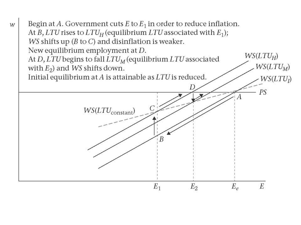
35. Hysteresis: Long-term unemployment Long-term unemployed effectively withdraw from the labour market due to progressive loss of skills and erosion of psychological attachment to working life (highly pertinent to South Africa’s “structural unemployment”) The higher is the ratio of long-term unemployed to the overall pool of unemployed the less impact has the level of U on wages => WS curve shifts upwards (for given E wages higher as long-term unemployed do not put downward pressure on wages) Hysteresis effect- emergence of long-term U leads to prolonged period of high U

36. Too few people work in South Africa 36 The employment to population ratio in South Africa and other emerging market economies Source: Statistics SA, ILO

37. Fig 4.9 At point A (with equil. employment Ee) AD falls (e.g. in SA Case investor confidence under apartheid is low / text = disinflation policy) and employment falls to E1 (after some time the share of long-term unemployed rises, therefore WS rises to WS(LTUh) move from B to C When govt wishes to raise AD again the new equilibirium level of employment is at E2 (point D) In the long-run, the economy will return to A again as at point D the share of long-term unemployed will begin to decline (given the increase in employment) and gradually the WS(LTUh) curve will begin to shift down to WS(LTUm) and then to WS(LTUi) If the scarring has been very serious (over decades) then active labour market measure may be required to reintegrate the long- term unemployed back into the market (eg re-training programmes, grants fro travel to job interviews, etc) The flatter (dashed) WS curve shows the WS cure where the share of long-term unemployed is constant – this WS curve intersects with the PS curve at the long-run ERU at A (but due to the fact the the share of long-term unemployed is not constant and WS shifts up the return to A takes longer i.e. is a more gradual process)

39. Hysteresis – capacity scrapping effects Working through the PS curve – depressed economic activity leads to the scrapping of capital stock When AD rises again there are high rates of capacity utilisation at higher unemployment rates Shown in Fig 4.10: – Due to reduced AD economy shifts from A to higher unemployment at E1 (at B) – then after prolonged period of higher U and capital stock scrapping when AD recovers then at point C the new equilibirium is associated with lower employment levels (at e2) – This is because when AD recovers and employment levels begin to rise (and wages fall) there is les capital stock for labour to work with – In longer-run economy will recover to A as higher capacity utilisation at C will stimulate investment in increased capital stock

41. 3.6 Conclusions from chapter If WS is pushed up or PS is pushed down then E falls and ERU rises WS is pushed up (and equilibrium output and employment fall): – When unemployment benefits become more generous – Unions have more power – legal rights of industrial action (or union density or collective bargaining coverage) – Unions exercise less wage restraint (collapse of wage accord) – There is more intermediate level wage setting (as opposed to centralised or decentralised) PS is pushed down and equilibrium output and employment fall), when: – Rise in the tax wedge – Rise in the price mark-up (when monopoly power rises) – Fall in productivity – A rise in real interest rates – More employment regulation (net of any productivity gains) How does the CB respond to such shocks (or supply side changes) in the IS-PC-MR model: – As ye changes the position of the MR line changes (as it intersects with (y’e; π T ) – The interest rate will overshoot if the CB is sluggish in its response to the supply side shock – Inflation will always remain a π T if the CB fully anticipates the supply side shock

43. 3.7The Nairu or natural rate of employment Ball and Mankiw propose a method for measuring how the Nairu shifts over time – Their conclusion for the US economy is that the Nairu was low in the 60’s, then rose and peaked in the late 1970’s and then declined into the 1990’s (see Figure 1) – In IS-PC-MR model: – 60’s ye high, Nairu low – 70’s ye low, Nairu high – 90’s ye high, Nairu low The authors then discuss what the causes of the shifting Nairu could be – They conclude that demographic issues and government policies play some role, as well as an important role for changes in productivity growth

44. Measuring shifts in the NAIRU Inflation – Unemployment I-U trade off: π = k – aU (Philips rels – see quote from Hume) Expectations augmented I-U trade off: π = πe – a(U – U*) (i.e. if π > πe, therefore U < U* i.e. high inflation is associated with low U) With supply shocks: π = πe – a(U – U*) + v (i.e. π > πe could be associated with oil price shock or exchange rate depreciation = v) (Also longer term shifts in U* means that stable inflation can be associated with lower levels of U)

45. Measuring NAIRU Authors make use of adaptive expectations: π = πt-1 – a(U – U*) + v (Justified on basis that inflation has followed a random walk in recent decades i.e. πt = πt-1+ ut (ut = random error term), therefore, system approximates optimal rational behaviour) Re-write as ∆π = aU* - aU + v Rearrange and divide by a: U* + v/a = U + ∆π/a Therefore, shift in U* + v/a can be computed on basis of observables U + ∆π/a (with U* representing long-run trends and v/a representing short-run shocks) Using a technique called Hodrick-Prescott Filter to estimate the Long-run trend in the series (Fig 1)

47. Causes of Shift in NAIRU US 1960 to 2000 NAIRU is found to be time varying (5.4% in the 1960, peaking at 6,8% in 1979 and declining to 4,9% in 2000). Why? Demographic explanation: – Changing composition of the labour force i.e. changes in sizes of groups with relatively high or low rates of unemployment can change the aggregate unemployment rate – e.g. increase of numbers of (relatively high unemployment) young workers before 1980 (baby boom generation) led to increase in NAIRU and decrease in numbers of young workers led to decrease in NAIRU after 1980 – But, if fixed weight is given to different demographic groups (Perry- weighted index - not adjusted according to labour force shares) i.e. what would have happened to the NAIRU if there had been no demographic shift, it is found that the impact of demographics shifts has been modest (Figure 2)

48. Impact of Government Policies Government disability and incarceration policies can also impact on the NAIRU e.g. if government policies cause people to leave the work force due to paying better disability benefits or due to increased incarceration then the NAIRU will tend to decline (as these people are removed from groups likely to experience high unemployment) Changing policies on disability and incarceration in the 80 ’ s and 90 ’ s could explain a reduction of the NAIRU by only about 0,8% (with disability policy playing a more important role with numbers rising from 3,1% of workforce in 1984 to 5,3% in 2000

49. Productivity Acceleration An approach is that rising productivity (e.g. growth of output per hour of work) is associated with a decline in the NAIRU (in the 1990 ’ s) and falling productivity is associated with an increase in the NAIRU ( “ productivity slowdown ” of the 1970 ’ s) Explained by the fact that “ wage aspirations ” adjust slowly to shifts in productivity growth – i.e. when productivity slumps real wages must fall, but this is resisted, real wages are relatively high and the NAIRU increases (in 1970’s λ falls => PS down while WS downward adjustment is sluggish so employment falls/NAIRU rises) – Or, when productivity accelerates, workers accustomed to slow wage growth, mean that real wages do not increase accordingly and employment levels rise, NAIRU falls (in 1990’s λ rises => PS rises while WS upward adjustment is sluggish so employment rises/NAIRU falls)

50. Explaining the 1990 ’ s What is important in explaining the fall of the NAIRU in the 1990 ’ s is not the rate of productivity growth (which was actually slightly higher in the 1960 ’ s than 1990 ’ s), but the increase in productivity relative to the recent past (i.e. the slowdown of the 1970 ’ s) Past experience meant that wage aspirations were not high when productivity increased in the 1990 ’ s, so adjustment was slow resulting effectively in a situation of a mismatch between productivity levels and real wages The 1990 ’ s experienced a period of falling unemployment and low inflation (reflected in reduction in the NAIRU)