1. MATCHING Eva Hromádková, 14.10.2010 Applied Econometrics JEM007, IES Lecture 4

2. Introduction “If I do not have experiment, how can I get control group?” Last time: Diff-in-diff  Comparison before-after between two comparable groups  Assumption: fixed differences between control and treatment group over time  How can we check / adjust assumption:  Look for trends in pre-treatment period  Selection into treatment based on temporary factors (Ashenfelter dip), or anticipation of treatment (taxes)

3. Matching Intuition  Counterfactuals: what would have happened to treated subjects, if the had not received treatment?  Potential (observed) outcomes x real outcomes Matching = pairing treatment and comparison units that are similar in terms of observable characteristics  Conditional on observables (X i ) we can take assignment to treatment (T i ) as “random” (unconfoundness)  Implicitly, unobservables do not play role in treatment assignment – we assume they are similar among groups

4. Matching Intuition II  E(Y 1 – Y 0 | T=1) = (1) E[Y 1 | X, T=1] – E[Y 0 | X, T=0] - (2) E[Y 0 | X, T=1] – E[Y 0 | X, T=0]  Part 1 is matched treatment effect  Part 2 is assumed to be zero  all selection occurs only through observed X

5. Matching Common support  Matching can only work if there is a region of “common support”  People with the same X values are in both the treatment and the control groups  Let S be the set of all observables X, then 0<Pr(T=1 | X)<1 for some S * subset of S  Intuition: Someone in control group has to be close enough to match to treatment unit, or we see enough overlap in the distribution of treated and untreated individuals over their characteristics

6. Matching Common support II

7. Matching methods Overview  Exact matching  Propensity score matching  Nearest neighbor  Kernel matching  Radius matching  Stratification matching

8. Exact matching  Each group of treated has her counterpart with exactly same characteristics  We define cells for combinations of observables E.g.: Sex x age x education x region  We compare average of treated and untreated in each cell (combination of characteristics)  Total effect: weighted average of cells (weights are frequencies of observed cells)  Example: Payne, Lissenburgh, White a Payne (1996)  Employment training, Employment Action in Great Britain  Treated: long term unemployed

9. Exact matching Issues Problem:  To create cells, only few X’s can be used  If we use more X’s, we will not have enough matches  Few X’s might not fully explain selection process => main assumption of matching would be violated  We need a tool that “merges” more dimensions into one  1 number – score, that would measure how much similar are treated and untreated  Solution = propensity score matching

10. Propensity score matching Explanation Propensity score = probability that an individual is treated based on his/her pre-treatment characteristics P(X) = P(T=1|X) = E(T|X) When can we use p(X) instead of X?  Balancing property – for given propensity score (range), distribution of characteristics of treated and untreated is the same (testable!!)  Unconfoundness - Conditional on observables (X i ) we can take assignment to treatment (T i ) as “random”

11. Propensity score matching General procedure 1-to-n Match  Nearest neighbor matching  Caliper matching  Nonparametric/kernel matching Run Logistic Regression: Dependent variable: T=1, if participate; T = 0, otherwise. Choose appropriate conditioning variables, X Obtain propensity score: predicted probability (p) Multivariate analysis based on new sample 1-to-1 match  Nearest neighbor matching  estimate difference in outcomes for each pair  Take average difference as treatment effect

12. Propensity score matching Step 1: Estimation of propensity score  Estimate logit or probit from the sample of treated and non-treated  Check balancing property (test means of X within stratas by p(X))  Choose common support

13. Propensity score matching Step 2: Matching algorithms A. Stratification:  Dividing range of propensity scores (PS) into intervals until we get the same average of PS for treated and untreated  In practice, this is NOT EASY  Within each intervals we compute difference in average outcome between treated and untreated  Weighting is based on number of units within a range

14. Propensity score matching Step 2: Matching algorithms B. Nearest neighbor method  Searching for the most similar unit between treated and control (closest propensity score)  Distance (difference of PS) between treated and control unit is not always same  All matches are weighted the same in final average effect C. Radius matching  We define distance and match with all controls within this distance – average of the effects (not weighted) D. Kernel matching  We put some type of distribution (e.g. normal) around the each treatment unit and use it to weight closer control units more and farther control units less  We can set “bandwith” - limiting the maximum distance in PS that is allowed

15. Propensity score matching Problems  Choice of matching algorithm – no “perfect” solution, depends on the properties of sample  Rule of thumb – if all give the same results it is ok, if not – look for problem  Standard errors: Estimated variance of treatment effect should include additional variance from estimating p  Typically people “bootstrap” which is a non-parametric form of estimating your coefficients over and over until you get a distribution of those coefficients—use the variance from that

16. Special topics in Propensity score matching PSM versus OLS  Why not doing simple OLS?  Common support – OLS extrapolated treatment effect also on the regions outside of common support  Implicit weighting differences: OLS is underweighting those combinations of Xs, where treatment or control group is dominant  Linear regression is imposing functional form, while PSM is nonparametric

17. Special topics in Propensity score matching PSM + DD  Worry that unobservables are causing selection because matching on X not sufficient  Can combine this with difference and difference estimates (Heckman’s procedure)  Obtain propensity score, construct control group J for each individual i  Estimate difference in outcome before treatment  If the groups are truly ‘as if’ random should be zero  If it’s not zero: can assume fixed differences over time and take before-after difference in treatment and control groups (DD)

18. Related literature Both on methods and applications: Caliendo and Kopeining (2008) – Some practical guidance for the implementation of propensity score matching Stuart (2010) – Matching methods for causal inference: A review and a look forward  Also includes Stata commands

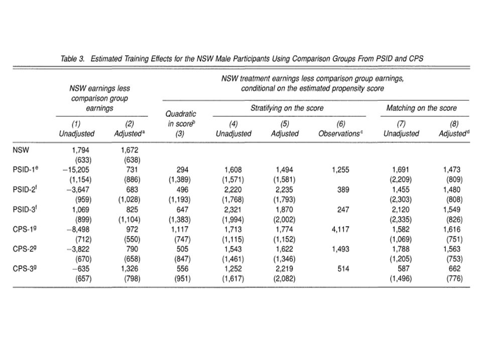
19. Can non-experimental methods (DD, matching) catch-up with experiments? LaLonde (1986) – NO Data: National Support Work Demonstration (NSW)  Help disadvantaged workers lacking basic skills  Duration of programme: 9-18 months  randomized into training versus no training !!! Goal of the study was to compare econometric estimates from those obtained from the experiment.  Use PSID and CPS to obtain control groups  Compare experimental to non-experimental estimates => Humbling experience for labor economists

21. Can non-experimental methods (DD, matching) catch-up with experiments? Further discussion  Dehejia and Wahba (1999, 2002) – YES  Same data  Propensity score matching, respect of common support (drop almost half of controls)  Includes only those with info on pre-program earnings  Smith and Lalonde (2005) - NO  DW results are sensitive to choice of Xs  Dehejia and Wahba (2006) – YES  Again stressing importance common support

23. Reality check  Questionable assumption about ignorability of unobservables in participation decision  Sensitive to what X we choose  Required to have a lot of pre-treatment (labor market behavior) and post-treatment characteristics  Good in evaluating obligatory programs or if filtering is based on some clearly define observed characteristics