1. Regional modeling of the Coastal Gulf of Alaska Albert J. Hermann (UW-JISAO/PMEL) I. Overview of modeling efforts and findings I. Overview of modeling efforts and findings –the importance of wind stress curl and localized tidal mixing –the essential role of iron in setting the cross-shelf spatial pattern of production II. Technical/mathematical challenges II. Technical/mathematical challenges –realistic parameterization of sub-gridscale estuaries and near- surface mixing

2. The Coastal Gulf of Alaska (CGOA) has complex bathymetry with submarine banks

3. Overview of Area Two major currents: Alaskan Stream and Alaska Coastal Current Two major currents: Alaskan Stream and Alaska Coastal Current ACC forced by downwelling-favorable winds and distributed runoff ACC forced by downwelling-favorable winds and distributed runoff Downwelling-favorable winds, yet very productive! Downwelling-favorable winds, yet very productive!

4. I. Overview of GOA modeling efforts (~past 5 years) and findings

5. UW/PMEL models (Hermann, Cheng et al.) ROMS at 10km and 3km resolution ROMS at 10km and 3km resolution Daily and 6-hourly atmos forcing Daily and 6-hourly atmos forcing Focus on nutrient flux, fish tracks Focus on nutrient flux, fish tracks

6. Nested model Sea Surface Salinity

7. Includes iron limitation (diagram from G. Gibson, UAF)

8. Focus on subregion of the CGOA DATA (summer climatology) MODEL (summer snapshot)

9. Modeled fluxes of no3 in the upper water column of the shelf indicate Patchy w with upwelling in the spring Patchy w with upwelling in the spring –unexpected since “downwelling favorable” coastal winds at this time – driven by CURL –Fiechter et al looked at interannual variability Vertical diffusion is the biggest term on the shelf as a whole – concentrated on seamounts (tidal mixing) Vertical diffusion is the biggest term on the shelf as a whole – concentrated on seamounts (tidal mixing)

10. Model output via Live Access Server: http://ferret.pmel.noaa.gov/foci

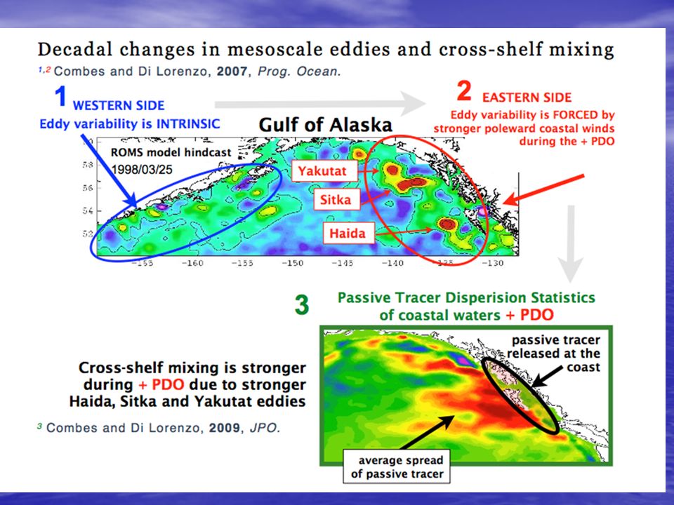
11. Georgia Tech Models (DiLorenzo, Combes, et al.) ROMS at 20km and 10 km resolution ROMS at 20km and 10 km resolution Monthly forcing Monthly forcing Focus on 200km eddies Focus on 200km eddies

13. UCSC models (Fiechter, Moore, et al.) ROMS at 10km resolution ROMS at 10km resolution Monthly forcing Monthly forcing Focus on data assimilation and interannual variability Focus on data assimilation and interannual variability

14. Coastal Gulf of Alaska Ocean Circulation Model ROMS: ~10 km horizontal resolution, 42 vertical levels One-way offline nesting with North East Pacific ROMS Monthly mean atmospheric and open boundary forcing Macro Nutrients from monthly WOA01 climatology Dissolved iron from VERTEX (Martin et al., 1989)

15. Lower Trophic Level Ecosystem Models NPZD+Fe (Powell et al., 2006; Fiechter et al., 2009) NPZD+Fe (Powell et al., 2006; Fiechter et al., 2009) NEMURO+Fe (Kishi et al., 2007; Fiechter and Moore, 2009) (from Kishi et al., 2007) Strom et al., 2007 NPZD PS: Nano P PL: Diatoms ZS: Ciliates ZL: Copepods ZP: Krill Fe

16. IS4DVAR Data Assimilation CASE NAME 7-DAY SSH (AVISO) 5-DAY SST (Pathfinder) IN SITU T/S (GLOBEC) 8-DAY CHL (SeaWiFS) FREENO SSHTYES NO SSHTP (AD, PASS)YES SSP (AD, PASS)NO YES Configuration: ROMS+NPZD+Fe, adjoint/passive biology Assimilation: 7-day cycle, 1 outer (NL) loop, 10 inner (TL/AD) loops Strong constraint (no model error), adjust IC only, model space search Univariate background error covariance: a) isotropic, homogeneous correlations (50km horiz., 30m vert.) b) std deviations based on 10-year non-assimilated solution Observation std deviations: SSH=2cm; T=0.25C; S=0.1; Chl=0.5mg/m 3

17. Physical data assim improves physics AND biology SSH CHL W/O ASSIMW/ASSIM

18. AOOS models (Chao et al.) ROMS nested at 9km/3km/1km ROMS nested at 9km/3km/1km Focus on PWS nowcast/forecast Focus on PWS nowcast/forecast

19. AOOS (from the AOOS website): AOOS will provide a centralized location for Data and information products from platforms such as buoys, providing wind and current speed and direction, wave height, sea temperature and salinity, and more; Data and information products from platforms such as buoys, providing wind and current speed and direction, wave height, sea temperature and salinity, and more; Enhancements to existing NOAA weather buoy data for specialized local needs; Enhancements to existing NOAA weather buoy data for specialized local needs; Processed satellite data providing Alaska-wide information on sea- surface temperature, ocean color (chlorophyll) and wind; Processed satellite data providing Alaska-wide information on sea- surface temperature, ocean color (chlorophyll) and wind; Geographically comprehensive surface current data from high frequency radar; Geographically comprehensive surface current data from high frequency radar; Data about fish, birds and marine mammals, the environmental effects of human activities, and any other information that can be used with the physical data to predict future changes to the ocean ecosystem. Data about fish, birds and marine mammals, the environmental effects of human activities, and any other information that can be used with the physical data to predict future changes to the ocean ecosystem.

20. End-to-End PWS Ocean Forecasting System Observatory data Deploy & Verify Models Data Assimilation Forecast Hypotheses Sensor & Platform Nowcast Questions

21. 1-km 3-km 9-km 21 Regional Ocean Modeling System (ROMS): 3-domain online nesting for Prince William Sound, AOOS Yi Chao, JPL & UCLAFrancois Colas & Jim McWilliams, UCLA

22. JPL ROMS Analysis & Forecast End-to-End Integration for Data and Models One-Stop Portal Yi Chao, JPL & UCLA ROMS real-time data assimilation and nowcast/forecast during a 2-week (July 2009) field experiment

23. 23 Surface drifters to evaluate the ROMS ensemble (16-member) forecast during the 2009 field experiment ObservationEnsemble Forecast Forecasting drifter trajectory Distance (km) 204060 Forecast Time (hour) Yi Chao, JPL & UCLA

24. 24 Coupled ROMS-NPZ modeling: Encouraging results with rooms for future improvements Yi Chao, JPL & UCLA Fei Chai, Univ. Maine

25. II. Technical challenges: sensitivity of the model to the specifics of line source buoyancy input at the coast

26. Nested ROMS and the GAK line

27. A simple salt-wedge estuary Diagrams courtesy of Pritchard Our nemesis: the runaway estuary effect -> freshwater penetrates horizontally -> vertical stratification increases -> mixing shuts down -> freshwater penetrates horizontally…

28. Four methods 1. Near-surface river 2. Dambreak river 3. Partially mixed deep estuary 4. Totally mixed shallow estuary

29. Method 5: tame the runaway estuary by spreading the source horizontally - as in global CCSM, apply runoff as near-coastal “rainfall” - use CCSM spatial pattern but sharpen to width of ACC - modulate in time using Royer’s (1982) hydrological model

30. Location of the GAK line

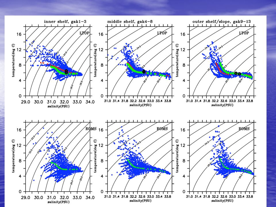
31. Modeled (ROMS) vs. measured (LTOP) T

32. Modeled (ROMS) vs. measured (LTOP) S

33. What is needed? (a subjective wish list) RUNOFF in space and time RUNOFF in space and time WINDS with orographic effects WINDS with orographic effects ICE DYNAMICS (needed for Cook Inlet) ICE DYNAMICS (needed for Cook Inlet) TIDES TIDES NUTRIENTS (most important bio IC/BC) NUTRIENTS (most important bio IC/BC) RESOLUTION of the estuaries RESOLUTION of the estuaries POST RESULTS ONLINE (e.g. DODS address) POST RESULTS ONLINE (e.g. DODS address)

34. Thanks to collaborators! N. Bond (UW-JISAO/PMEL) W. Cheng (UW-JISAO/PMEL) K. Coyle (UAF) E. N. Curchitser (Rutgers U.) E. DiLorenzo (GaTech) E. L. Dobbins (UW-JISAO/PMEL) J. Fiechter (UCSC) G. Gibson (UAF) D. B. Haidvogel (Rutgers U.) K. Hedstrom (ARSC) S. Hinckley (NOAA/AFSC) N. Kachel (UW-JISAO/PMEL) A. Moore (UCSC) C. Mordy (UW-JISAO/PMEL) T. Powell (UC-Berkeley) P. J. Stabeno (NOAA/PMEL) R. Steed (UW)

35. FIN!

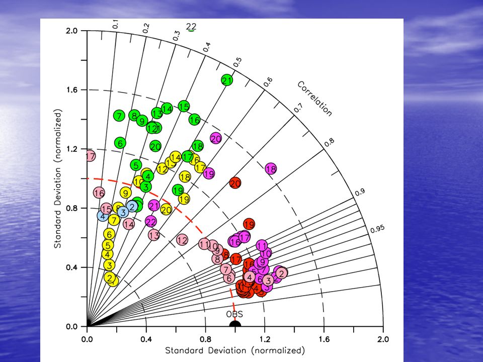
36. NPZD Surface Chlorophyll, 2001 Taylor diagrams with respect to SeaWiFS based on monthly means NO BIO ASSIM PASSIVE BIO ASSIM ADJOINT BIO ASSIM

37. Observed cross-shelf hydrography at the GAK line (data from Weingartner et al.)

38. AOOS is User-Dr iven Stakeholder concerns Climate change impacts Increased coastal erosion Changing marine ecosystems Unstable sea ice and uncertain freeze/thaw dates Fewer subsistence resources More shipping = more oil spill potential Changing sea state: more fog, storms, winds, waves Information Products Needed Nowcasts Warnings & bulletins Forecasts Weekly, monthly & seasonal outlooks Futurecasts Scenarios & projections Satellites Fixed platforms Ships Drifters Floats AUVs Observations Standards Data discovery Data transport Online browsing Data archive Data Management Integration & Analysis Outcomes: Meeting Societal Goals

39. Model–based findings: Physical sources for nitrate Horizontal advection Horizontal advection Vertical advection Vertical advection Vertical diffusion Vertical diffusion Seek to quantify these basic terms across the faces of a control volume Seek to quantify these basic terms across the faces of a control volume Note: result depends on the dimensions of the box! Note: result depends on the dimensions of the box! Adv in from E Adv out to W Adv in from basin Vert adv N N

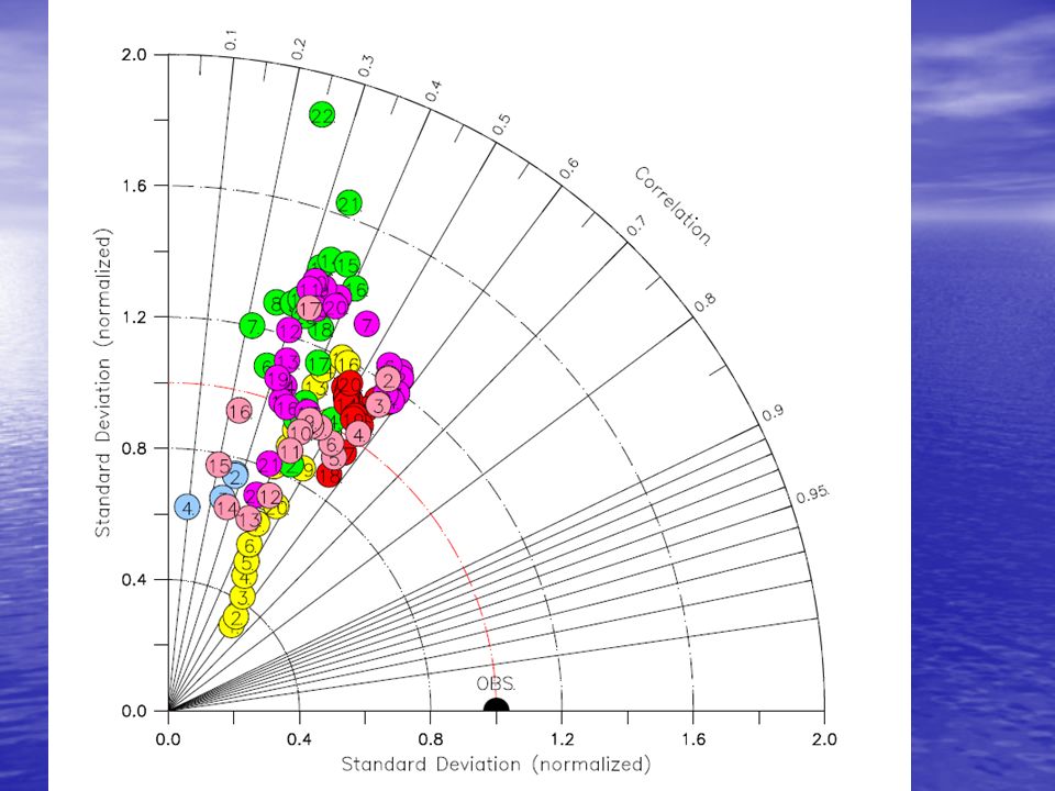
40. Modled vs. measured EKE

41. Model overview Regional Ocean Modeling System (ROMS) Regional Ocean Modeling System (ROMS) 3km grid, 42 vertical levels 3km grid, 42 vertical levels LMD mixed layer physics LMD mixed layer physics wind and heat forcing: wind and heat forcing: –NCEP/CORE2/MM5 ICs/BCs ICs/BCs –ROMS-NEP5 (Curchitser and Hedstrom)/SODA Coupled to NPZ and IBMs Coupled to NPZ and IBMs Results posted on Live Access Server Results posted on Live Access Server Used in various biophysical programs: Used in various biophysical programs: –Eco-FOCI, GLOBEC, GOA-IERP,…..

42. ROMS Nested Modeling 12-km 1-km 3-km Multi-scale (or “nested”) ROMS modeling approach is developed in order to simulate the 3D ocean at the spatial scale (e.g., 1- km) measured by in situ and remote sensors From Pacific to Gulf of Alaska, and to PWS offline online

43. Modeled cross-shelf salinity: partial success but still “runaway estuary”

44. What is still missing? Surface wave breaking Surface wave breaking Langmuir cells Langmuir cells True estuarine physics! True estuarine physics!

45. New forcing scheme retains flux through Shelikof Strait… Data Method 4 Method 5

46. ..and yields a nice match with temperature data….

47. ..and a nice match with salinity data (but miss the freshest water at the coast)

50. Jerome Fiechter, Andy Moore, Gregoire Broquet Ocean Sciences Department University of California, Santa Cruz ROMS Workshop, Sydney, April 2009 Improving Ecosystem Model Predictions through Data Assimilation

53. Inter-annual variability: higher salinity in 2002

54. Inter-annual variability: lower SSH in 2002

55. May 2002: weak ACC, more cross-shelf flow

56. May 2003: strong ACC, less cross-shelf flow

57. Monthly average wind stress vectors (N m -2 ) and wind stress curl (N m -3 x 10 3, shaded) May 2001 Aug 2001

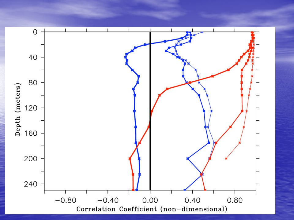
58. Calculated Ekman pumping from winds (black line) vs ROMS vertical velocities at 15 m (red line) integrated over the control volume

59. Modeled monthly average horizontal flux of nitrate at 15 m depth (millimole m -2 s -1 ) May 15 2001Aug 15 2001

60. May 2001 average vertical advection and vertical diffusion of nitrogen across the 15m depth horizon (millimole m -2 s -1 x 10 3 ) VERTICAL ADVECTIONVERTICAL DIFFUSION

61. NO3 flux summary (unfiltered) Fortnightly tidal period drives fortnightly mixing

62. First, look at the water budget: upwelling in spring, onshore flux Adv in from E Adv in from basin Vert adv Sum of adv Adv out to W

63. Ongoing/future directions Data assimilation (Fiechter, Moore et al.) Data assimilation (Fiechter, Moore et al.) Finer grids – resolve the estuaries! Finer grids – resolve the estuaries! –But note some artifacts (e.g. runaway estuary) do not get better at high resolution Bigger ensembles Bigger ensembles –Vary parameters –Vary ICs, BCs Combined IBM/Eulerian approaches Combined IBM/Eulerian approaches

64. Nested ROMS and the GAK line

65. Nitrate flux summary (30-d lowpass) Vert diff Sum of adv Vert adv Adv in from basin Adv out to W Adv in from E