1. Portfolio risk and return
Return Generating model, Beta, CAPM and SML
9/23/15 1

2. Return Generating models
Used to estimate the expected returns on risky securities based on specific factors
For each security, we must estimate the sensitivity of its returns to each specific factor
Factors that explain security returns can be classified as
macroeconomic,
fundamental, and
statistical factors.
9/23/15 2

3. Multifactor models most commonly use macroeconomic factors such as GDP growth, inflation, or consumer confidence, along with
fundamental factors such as earnings, earnings growth, firm size, and research expenditures.
Statistical factors often have no basis in finance theory and are suspect in that they may represent only relations for a specific time period which have been identified by data mining

4. The general form of a multifactor model with k factors

5. This model states that the expected excess return (above the risk-free rate) for Asset i is
the sum of each factor sensitivity or factor loading for Asset i multiplied by the expected value of that factor for the period.
The first factor is often the expected excess return on the market, E(Rm - Rf).

6. Fama- French model
They estimated the sensitivity of security returns to three factors:
firm size,
firm book value to market value ratio, and
the return on the market portfolio minus the risk-free rate (excess return on the market portfolio).
price momentum using prior period returns (Carhart)

7. The simplest factor model is a single- factor model with the return on the market, Rm , as its only risk factor (single-index model.)

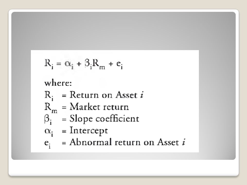
8. Market model A simplified form of a single-index model
It’s used to estimate a security’s (or portfolio’s) beta and to estimate a security’s abnormal return (return above its expected return) based on the actual market return.

10. slope coefficient ( ) the security beta
Intercept of this equation ( )is the security’s expected excess return when the market excess return is zero
slope coefficient ( ) the security beta
It is the amount by which the security return tends to increase or decrease for every 1% increase or decrease in the return on the index
is the error term firm-specific surprise in the security return in time t, also called the residual.

11. Expected return on Asset i is
A deviation from the expected return in a given period is the abnormal return on Asset
In the market model, the factor sensitivity or beta for Asset i is a measure of how sensitive the return on Asset i is to the return on the overall market portfolio (market index).

12. 2nd term to the equation is the systematic risk premium/market risk premium because it derives from the risk premium that characterizes the entire market.
1st term to the equation ( ) nonmarket premium; may be large if you think a security is underpriced and therefore offers an attractive expected return.
Superior analysis; finding securities that have non-zero values of alpha.

13. Calculating beta
We have concluded in the previous session that the only relevant risk of a particular asset is its systematic risk, that is, the sensitivity of its returns to changes in the overall market.
This sensitivity is measured as the covariance of the asset’s return with the market return
This covariance is standardized by dividing the covariance by the market variance
9/23/15 13

14. 9/23/15 14

15. We can use the definition of the correlation between the returns on Asset i with the returns on the market index:
Substituting for Covim in the equation for Bi, we can also calculate beta as:
9/23/15 15

16. Total risk = Systematic risk + Firm-specific risk

17. Concept check
The standard deviation of the return on the market index is estimated as 20%.
If Asset A’s standard deviation is 30% and its correlation of returns with the market index is 0.8, what is Asset A’s beta?
If the covariance of Asset A’s returns with the returns on the market index is 0.048, what is the beta of Asset A?
9/23/15 17

18. The slope of the least squares regression line is beta
In practice, we estimate asset betas with a regression of the returns on the asset over some period on those of the market index
Asset returns are the dependent variable and the returns on the market index are the independent variable.
The slope of the least squares regression line is beta
9/23/15 18

19. Regression of Asset Excess Returns against Market Asset Returns
9/23/15 19

20. This regression line is referred to as the asset’s (security) characteristic line.
Mathematically, the slope of the characteristic line is the same formula we used earlier to calculate beta.
9/23/15 20

21. Class exercise (4 minutes)
The covariance of the market’s returns with a stock’s returns is and the standard deviation of the market’s returns is What is the stock’s beta?
The covariance of the market’s returns with the stock’s returns is The standard deviation of the market’s returns is 0.08 and the standard deviation of the stock’s returns is What is the correlation coefficient of the returns of the stock and the returns of the market?
9/23/15 21

22. Case of HP; Regression analysis

23. ANOVA Table

24. The sum of squares (SS) of the regression (
The sum of squares (SS) of the regression (.3752) is the portion of the variance of the dependent variable (HP’s return) that is explained by the independent variable (the S&P 500 return)
The MS column for the residual (.0059) shows the variance of the unexplained portion of HP’s return, that is, the portion of return that is independent of the market index
Square root of this value is the standard error (SE) of the regression (.0767)

25. The table shows the beta estimate for HP to be 2
The table shows the beta estimate for HP to be , more than twice that of the S&P 500.
SE produce a large t -statistic (7.9888), and a p -value of practically zero; we can confidently reject the hypothesis that HP’s true beta is zero i.e. statistical significance
standard deviation of HP’s residual is 7.67%, or 26.6% annually
The standard deviation of systematic risk is beta* std.dev (market) 27.57% (2.0348*13.)

26. R -square (the ratio of explained to total variance) equals the explained (regression) SS divided by the total SS
= (.3752/.7162 * 100%)

27. CAPM and SML
Given that the only relevant (priced) risk for an individual Asset i is measured by the covariance between the asset’s returns and the returns on the market, Cov i,mkt, we can plot the relationship between risk and return for individual assets using Cov i,mkt as our measure of systematic risk.
The resulting line, plotted in the next slide, is one version of what is referred to as the security market line (SML).
9/23/15 27

28. Security Market Line
9/23/15 28

29. The equation of the SML is: which can be rearranged and stated as:
But the covariance between the security and the market divided by the market variance is beta. So we can substitute beta for the covariance expression (RFR is risk free rate)
9/23/15 29

30. Formally, the CAPM is stated as:
This is the most common means of describing the SML, and this relation between beta (systematic risk) and expected return is known as the capital asset pricing model (CAPM).
Formally, the CAPM is stated as:
Beta is a standardized measure of systematic risk.
Beta measures the relation between a security’s excess returns and the excess returns to the market portfolio.
9/23/15 30

31. CAPM
9/23/15 31

32. We repeat: Beta measures systematic (market or covariance) risk.
The CAPM holds that, in equilibrium, the expected return on risky asset E(Ri) is the risk-free rate (Rf) plus a beta-adjusted market risk premium, bi[E(Rmkt) – Rf ].
We repeat: Beta measures systematic (market or covariance) risk.
9/23/15 32

33. If the beta is less than 1 it has less risk than the market portfolio
If a security has a beta of 1 it has the same risk as the market portfolio
If the beta is less than 1 it has less risk than the market portfolio
If beta is greater than 1 the security has a higher risk than the market
9/23/15 33

34. Comparing the CML and the SML
9/23/15 34

35. The SML:
9/23/15 35

36. The CML uses total risk = Standard deviation of portfolio on the X-axis. Hence, only efficient portfolios will plot on the CML.
On the other hand, the SML uses beta (systematic risk) on the X-axis. So in a CAPM world, all properly priced securities and portfolios of securities will plot on the SML
9/23/15 36

37. Portfolios that are not well-diversified (efficient) plot inside the efficient frontier and are represented by risk-return combinations such as points A, B, and C in panel (a) of the CML graph. Individual securities are one example of such inefficient portfolios.
According to the CAPM, the expected returns on all portfolios, well-diversified or not, are determined by their systematic risk.
9/23/15 37

38. Thus, according to the CAPM, Point A represents a high-beta stock or portfolio, point B a stock or portfolio with a beta of one, and point C a low-beta stock or portfolio.
We know this because the expected return at Point B is equal to the expected return on the market, and the expected returns at Point A and C are greater and less than the expected return on the market (tangency) portfolio, respectively.
Therefore according to the CAPM, all securities and portfolios, diversified or not, will plot on the SML in equilibrium.
9/23/15 38

39. Calculate and interpret the expected return of an asset using the CAPM.
The CAPM is one of the most fundamental concepts in investment theory.
The CAPM is an equilibrium model that predicts the expected return on a stock, given the expected return on the market, the stock’s beta coefficient, and the risk-free rate.
Remember CAPM is the equation of the SML
9/23/15 39

40. Examples
The expected return on the market is 15%, the risk-free rate is 8%, and the beta for Stock A is 1.2. Compute the rate of return that would be expected (required) on this stock.
The expected return on the market is 15%, the risk-free rate is 8%, and the beta for Stock B is 0.8. Compute the rate of return that would be expected (required) on this stock.
9/23/15 40

41. Applications of the CAPM and the SML
We can use CAPM to determine a security’s required rate of return and also to determine whether a security is overvalued or undervalued
Example: A ltd has a capital structure that is 40% debt and 60% equity. The expected return on the market is 12%, and the risk-free rate is 4%. What discount rate should an analyst use to calculate the NPV of a project with an equity beta of 0.9 if the firm’s after-tax cost of debt is 5%?
9/23/15 41

42. Illustration
The following figure contains information based on analyst’s forecasts for three stocks.
Assume a risk-free rate of 7% and a market return of 15%. Compute the expected and required return on each stock, determine whether each stock is undervalued, overvalued, or properly valued, and outline an appropriate trading strategy.
9/23/15 42

43. Identifying Mispriced Securities
9/23/15 43

45. All securities that plot above the SML are underpriced as investors are expecting a higher rate of return than they should for an asset of that particular risk return characteristics
Similarly, all securities that plot below the SML are overpriced for the same reason only that they are expecting a lower rate of return than they should
9/23/15 45

46. Key Differences Between the SML and the CML
9/23/15 46