1. Helmholtz-Instituts für Strahlen- und Kernphysik J. Ruiz de Elvira Precise dispersive analysis of the f0(500) and f0(980) resonances R. García Martín, R. Kaminski, J. R. Peláez, JRE, Phys.Rev. Lett. 107, 072001 (2011) R. García Martín, R. Kaminski, J. R. Peláez, JRE, F. J. Yndurain. PRD83,074004 (2011)

2. Motivation: The f 0 (500)/ σ and the f 0 (980) I=0, J=0  exchange very important for nucleon-nucleon attraction Scalar multiplet identification still controversial EFT: Chiral symmetry breaking. Vacuum quantum numbers. Role on values of chiral parameters. Similarities and differences with EW-Higgs boson. Strongly interacting EWSBS.  f0f0 a0a0 All these states do mix Too many scalar resonances below 2 GeV. Possible exotic nature: tetraquarks,molecules,glueballs… Glueball search: Characteristic feature of non-abelian QCD nature

3. Motivation: The f 0 (500) controversy until 2012 Very controversial since the 60’s. The reason: The f 0 (500) is a EXTREMELY WIDE. Usually refereed to its pole: Mostly “observed” in  scattering, but no “resonance peak”. After 2000 also observed in Dalitz plots in production process “not well established” 0 + state in PDG until 1974 Removed from 1976 until 1994. Back in PDG in 1996 PDG2002: “σ well established” However, since 1996 still quoted as Mass= 400-1200 MeV Width= 600-1000 MeV

4. 1987 1979 1973 1972 Most confusion due to using MODELS (with questionable analytic properties)

5. It is model independent. Just analyticity and crossing properties Motivation: Why a dispersive approach? Determine the amplitude at a given energy even if there were no data precisely at that energy. Relate different processes Increase the precision The actual parametrization of the data is irrelevant once it is used in the integral. A precise  scattering analysis can help determining the  and f0(980) parameters

6. Data after 2000 both scattering and production Dispersive- model independent approaches Chiral symmetry correct

7. OUR AIM Precise DETERMINATION of f 0 (500) and f0(980) pole FROM DATA ANALYSIS Use of Roy and GKPY dispersion relations for the analytic continuation to the complex plane. (Model independent approach) Use of dispersion relations to constrain the data fits (CFD) Complete isospin set of Forward Dispersion Relations up to 1420 MeV Up to F waves included Standard Roy Eqs up to 1100 MeV, for S0, P and S2 waves Once-subtracted Roy like Eqs (GKPY) up to 1100 MeV for S0, P and S2 We do not use the ChPT predictions. Our result is independent of ChPT results. Essential for f 0 (980)

8. Roy Eqs. vs. Forward Dispersion Relations FORWARD DISPERSION RELATIONS (FDRs). (Kaminski, Pelaez and Yndurain) One equation per amplitude. Positivity in the integrand contributions, good for precision. Calculated up to 1400 MeV One subtraction for F00 and F0+ FDR No subtraction for the It=1FDR. They both cover the complete isospin basis

9. Forward dispersion relations Used to check the consistency of each set with the other waves Contrary to Roy. eqs. no large unknown t behavior needed Complete set of 3 forward dispersion relations: Two symmetric amplitudes. F 0+   0  +  0  +, F 00  0  0  0  0 Only depend on two isospin states. Positivity of imaginary part Can also be evaluated at s=2M  2 (to fix Adler zeros later) The I t =1 antisymmetric amplitude At threshold is the Olsson sum rule Below 1450 MeV we use our partial wave fits to data. Above 1450 MeV we use Regge fits to data.

10. Roy Eqs. vs. Forward Dispersion Relations FORWARD DISPERSION RELATIONS (FDRs). (Kaminski, Pelaez and Yndurain) One equation per amplitude. Positivity in the integrand contributions, good for precision. Calculated up to 1400 MeV One subtraction for F00 and F0+ FDR No subtraction for the It=1FDR. ROY EQS (1972) (Roy, M. Pennington, Caprini et al., Ananthanarayan et al. Gasser et al.,Stern et al., Kaminski. Pelaez,,Yndurain). Coupled equations for all partial waves. Limited to ~ 1.1 GeV. Twice substracted. Good at low energies, interesting for ChPT. When combined with ChPT precise for f0(500) pole determinations. (Caprini et al) But we here do NOT use ChPT, our results are just a data analysis They both cover the complete isospin basis

11. NEW ROY-LIKE EQS. WITH ONE SUBTRACTION, (GKPY EQS) When S.M.Roy derived his equations he used. TWO SUBTRACTIONS. Very good for low energy region: In fixed-t dispersion relations at high energies : if symmetric the u and s cut (Pomeron) growth cancels. if antisymmetric dominated by rho exchange (softer). ONE SUBTRACTION also allowed GKPY Eqs. But no need for it!

12. Structure of calculation: Example Roy and GKPY Eqs. Both are coupled channel equations for the infinite partial waves: I=isospin 0,1,2, l =angular momentum 1,2,3…. Partial wave on real axis SUBTRACTION TERMS (polynomials) KERNEL TERMS known 2nd order 1st order More energy suppressed Less energy suppressed Very small small ROY: GKPY: DRIVING TERMS (truncation) Higher waves and High energy “IN (from our data parametrizations)” “OUT” =? Similar Procedure for FDRs

13. UNCERTAINTIES IN Standard ROY EQS. vs GKPY Eqs smaller uncertainty below ~ 400 MeVsmaller uncertainty above ~400 MeV Why are GKPY Eqs. relevant? One subtraction yields better accuracy in √s > 400 MeV region Roy Eqs.GKPY Eqs,

14. ROY vs. GKPY Eqs. Roy Eqs. Require HUGE cancellations between terms above 400 MeV Both KT and ST are FAR LARGER than UNITARITY BOUNDS GKPY do not Note the difference In scale!!

15. ROY vs. GKPY Eqs. This the real proportion

16. Our series of works: 2005-2011 Independent and simple fits to data in different channels. “Unconstrained Data Fits UDF” Check Dispersion Relations Impose FDRs, Roy Eqs and Sum Rules on data fits “Constrained Data Fits CDF” Describe data and are consistent with Dispersion relations Some data sets inconsistent with FDRs All waves uncorrelated. Easy to change or add new data when available Some data fits fair agreement with FDRs Correlated fit to all waves satisfying FDRs. precise and reliable predictions. from DATA unitarity and analyticity R. Kaminski, JRP, F.J. Ynduráin Eur.Phys.J.A31:479-484,2007. PRD74:014001,2006 J. R. P,F.J. Ynduráin. PRD71, 074016 (2005), PRD69,114001 (2004), R. García Martín, R. Kaminski, JRP, J. Ruiz de Elvira, F.J. Yduráin 2011, PRD83,074004 (2011) Continuation to complex plane USING THE DISPERIVE INTEGRALS: resonance poles

17. The fits 1)Unconstrained data fits (UDF) All waves uncorrelated. Easy to change or add new data when available The particular choice of parametrization is almost IRRELEVANT once inside the integrals we use SIMPLE and easy to implement PARAMETRIZATIONS.

18. S0 wave below 850 MeV Conformal expansion, 4 terms are enough. First, Adler zero at m  2 /2 We use data on Kl4 including the NEWEST: NA48/2 results Get rid of K → 2  Isospin corrections from Gasser to NA48/2 Average of  N->  N data sets with enlarged errors, at 870- 970 MeV, where they are consistent within 10 o to 15 o error. Tiny uncertainties due to NA48/2 data It does NOT HAVE A BREIT-WIGNER SHAPE

19. S0 wave above 850 MeV Paticular care on the f0(980) region : Continuous and differentiable matching between parametrizations Above1 GeV, all sources of inelasticity included (consistently with data) Two scenarios studied CERN-Munich phases with and without polarized beams Inelasticity from several   ,   KK experiments

20. S0 wave: Unconstrained fit to data (UFD)

21. Similar Initial UNconstrained FIts for all other waves and High energies R. Kaminski, J.R.Pelaez, F.J. Ynduráin. Phys. Rev. D77:054015,2008. Eur.Phys.J.A31:479-484,2007, PRD74:014001,2006 J.R.Pelaez, F.J. Ynduráin. PRD71, 074016 (2005), From older works:

22. UNconstrained Fits for High energies J.R. Pelaez, F.J.Ynduráin. PRD69,114001 (2004) UDF from older works and Regge parametrizations of data Factorization In principle any parametrization of data is fine. For simplicity we use

23. The fits 1)Unconstrained data fits (UDF) Independent and simple fits to data in different channels. All waves uncorrelated. Easy to change or add new data when available Check of FDR’s Roy and other sum rules.

24. How well the Dispersion Relations are satisfied by unconstrained fits We define an averaged  2 over these points, that we call d 2 For each 25 MeV we look at the difference between both sides of the FDR, Roy or GKPY that should be ZERO within errors. d 2 close to 1 means that the relation is well satisfied d 2 >> 1 means the data set is inconsistent with the relation. There are 3 independent FDR’s, 3 Roy Eqs and 3 GKPY Eqs.

25. Forward Dispersion Relations for UNCONSTRAINED fits FDRs averaged d 2  0  0 0.31 2.13  0  + 1.03 1.11 I t =1 1.62 2.69 <932MeV <1400MeV NOT GOOD! In the intermediate region. Need improvement

26. Roy Eqs. for UNCONSTRAINED fits Roy Eqs. averaged d 2 GOOD! But room for improvement S0wave 0.64 0.56 P wave 0.79 0.69 S2 wave 1.35 1.37 <932MeV <1100MeV

27. GKPY Eqs. for UNCONSTRAINED fits Roy Eqs. averaged d 2 PRETTY BAD!. Need improvement. S0wave 1.78 2.42 P wave 2.44 2.13 S2 wave 1.19 1.14 <932MeV <1100MeV GKPY Eqs are much stricter Lots of room for improvement

28. Lesson to learn: Despite using Very reasonable parametrizations with lots of nice properties, obtaining nice looking fits to data… They are at odds with FIRST PRINCIPLES crossing, causality (analyticity)… And of course, to extrapolate to the complex plane ANALYTICITY is essential

29. The fits 1)Unconstrained data fits (UDF) Independent and simple fits to data in different channels. All waves uncorrelated. Easy to change or add new data when available Check of FDR’s Roy and other sum rules. Room for improvement 2) Constrained data fits (CDF)

30. Imposing FDR’s, Roy Eqs and GKPY as constraints To improve our fits, we can IMPOSE FDR’s, Roy Eqs. W roughly counts the number of effective degrees of freedom (sometimes we add weight on certain energy regions) The resulting fits differ by less than ~1  -1.5  from original unconstrained fits The 3 independent FDR’s, 3 Roy Eqs + 3 GKPY Eqs very well satisfied 3 FDR’s 3 GKPY Eqs. Sum Rules for crossing Parameters of the unconstrained data fits 3 Roy Eqs. We obtain CONSTRAINED FITS TO DATA (CFD) by minimizing: and GKPY Eqs.

31. Forward Dispersion Relations for CONSTRAINED fits FDRs averaged d 2  0  0 0.32 0.51  0  + 0.33 0.43 I t =1 0.06 0.25 <932MeV <1400MeV

32. Roy Eqs. for CONSTRAINED fits Roy Eqs. averaged d 2 S0wave 0.02 0.04 P wave 0.04 0.12 S2 wave 0.21 0.26 <932MeV <1100MeV

33. GKPY Eqs. for CONSTRAINED fits Roy Eqs. averaged d 2 S0wave 0.23 0.24 P wave 0.68 0.60 S2 wave 0.12 0.11 <932MeV <1100MeV

34. Despite the remarkable improvement the CFD are not far from the UFD and the data is still welll described…

35. S0 wave: from UFD to CFD Only sizable change in f0(980) region

36. S0 wave: from UFD to CFD As expected, the wave suffering the largest change is the D2

37. DIP vs NO DIP inelasticity scenarios Longstanding controversy for inelasticity : (Pennington, Bugg, Zou, Achasov….) There are inconsistent data sets for the inelasticity... whereas the other one does notSome of them prefer a “dip” structure…

38. DIP vs NO DIP inelasticity scenarios Dip 6.15 No dip 23.68 992MeV< e <1100MeV UFD Dip 1.02 No dip 3.49 850MeV< e <1050MeV CFD GKPY S0 wave d 2 Now we find large differences in No dip ( forced) 2.06 Improvement possible? No dip (enlarged errors) 1.66 But becomes the “Dip” solution Other waves worse and data on phase NOT described

39. Analytic continuation to the complex plane We do NOT obtain the poles directly from the constrained parametrizations, which are used only as an input for the dispersion relations. The σ and f0(980) poles and residues are obtained from the DISPERSION RELATIONS extended to the complex plane. This is parametrization and model independent. Now, good description up to 1100 MeV. We can calculate in the f0(980) region. Effect of the f0(980) on the f0(500) under control. Residues from: or residue theorem

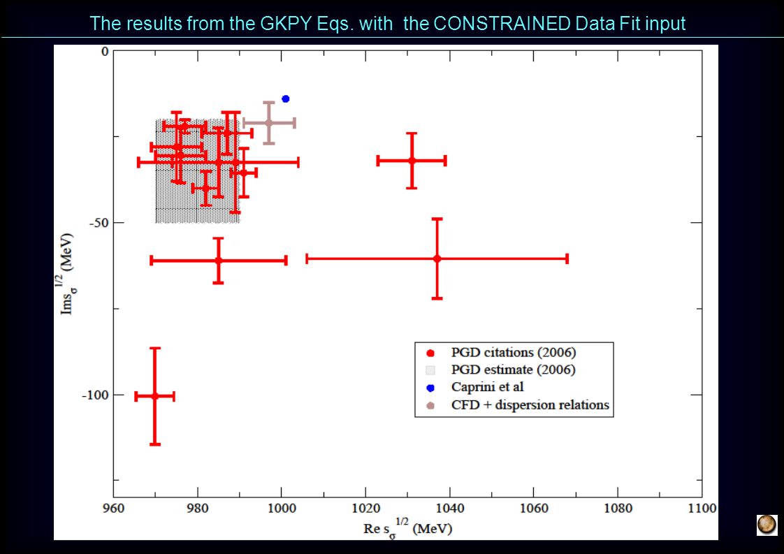
40. Final Result: Analytic continuation to the complex plane Roy Eqs. Pole: Residue: GKPY Eqs. pole: Residue: f0(500) f0(980) We also obtain the ρ pole: Fairly consistent with other ChPT+dispersive results Caprini, Colangelo, Leutwyler 2006 1  overlap with

41. Fairly consistent with other ChPT+dispersive results: Caprini, Colangelo, Leutwyler 2006 1  overlap with Final Result: discussion Falls in te bullpark of every other dispersive result.

42. The results from the GKPY Eqs. with the CONSTRAINED Data Fit input

44. Summary Simple and easy to use parametrizations fitted to  scattering DATA for S,P,D,F waves up to 1400 MeV. (Unconstrained data fits) Simple and easy to use parametrizations fitted to  scattering DATA CONSTRAINED by FDR’s+ Roy Eqs+ 3 GKPY Eqs 3 Forward Dispersion relations and the 3 Roy Eqs and 3 GKPY Eqs satisfied remarkably well We obtain the σ and f0(980) poles from DISPERSION RELATIONS extended to the complex plane, without use ChPT. The poles obtained are fairly consistents whit previous ones, but are obtained within a model independent precise analysis of the latest data “Dip scenario” for inelasticity favored

45. Epilogue Actually, after our work was published, the PDG 2012 edition made a major revision of the σ and f0(980).

46. PDG σ estimate until 2012

47. PDG 2012 revision for the σ53

48. PDG f0(980) estimate until 2012

49. PDG 2012 revision for the f0(980)

50. THANK YOU

51. SPARE SLIDES

52. Epilogue “One might also take the more radical point of view and just average the most advanced dispersive analyses, for they provide a determination of the pole positions with minimal bias. This procedure leads to the much more restricted range of f0(500) parameters” “One might also take the more radical point of view and just average the most advanced dispersive analyses, for they provide a determination of the pole positions with minimal bias. This procedure leads to the much more restricted range of f0(500) parameters” “Note on scalar mesons PDG2012”

53. The results from the GKPY Eqs. with the CONSTRAINED Data Fit input MotivationNature Properties SSB Conclusions Poles 55 Jacobo Ruiz de Elvira Carrascal Doctoral Dissertation Poles: PDG 2012 revision for the σ

54. Epilogue 56 Jacobo Ruiz de Elvira Carrascal Doctoral Dissertation “In this issue we extended the allowed range of the f0(980) mass to include the mass value derived in Ref. 10. We now quote for the mass” “Note on scalar mesons PDG2012”

55. Fairly consistent with other ChPT+dispersive results: Caprini, Colangelo, Leutwyler 2006 1  overlap with The existence of two kaon thresholds is relevant for the f0(980). We have repeated the UFD to CFD process for the two extreme cases and added half the difference as a systematic uncertainty. It is only relevant for the f0 width and amounts to 4 MeV Final Result: discussion and in general with every other dispersive result.

56. We can now use sum rules to obtain threshold parameters: We use the Froissart Gribov representantion, Olsson sum rule, and a couple of other sum rules we have derived Threshold parameters

57. We START by parametrizing the data To avoid model dependences we only require analyticity and unitarity We use an effective range formalism: s 0 =1450 +a conformal expansion If needed we explicitly factorize a value where f(s) is imaginary or has an Adler zero: For the integrals any data parametrization could do. We use something SIMPLE at low energies (usually <850 MeV) ON THE REAL ELASTIC AXIS this function coincides with cot δ

58. 1)The left cut lies rigth on |w|=1. 2)The KK cut lies rigth on |w|=1. Both cannot be described with the truncated conformal expansion One has to get used to thinking in terms of the w variable, that deforms considerably the complex plane, and recall that the expansion is convergent in w, not in s. For example, s=0 is outside the inner disk Our expresions cannot be used in any of those places. If one does, one very likely gets nonsense These points may look close to threshold, but they are not in terms of w.

59. Where do we expect it to converge with few parameters? Of course, we cannot use the full series. So, we have to truncate it. How many parameters we need? The  2 will tell us. As before, we have to stay far from the borders of the circle. For instance, the Adler zero comes out right since it is put there by hand, but w=-0.82, Beyond that we are too close to the border, and a truncated expansion may be bad. In particular one can get spurious poles with that particular parametrization. as noted by Caprini, Colangelo, Gasser Leutwyler Again one has the systematic uncertainty of the term one is dropping.

60. But the NA48/2 data falls very much inside the circle: barycenters between w=-0.537 and -0.401

61. We can for instance include compatible data points here, with large uncertainties

62. To avoid coming close to the edges of the circle s<(0.85 GeV) 2 and we use FOUR terms in the expansion k 2 and k 3 are kaon and eta CM momenta Imposing continuous derivative matching at 0.85 GeV, two parameters fixed In terms of δ and δ’ at the matching point S0 wave parametrization: details

63. s>(2 M k ) 2 Thus, we are neglecting multipion states but ONLY below KK threshold But the elasticity is independent of the phase, so… it is not necessarily only due to KKbar, (contrary to a 2 channel K matrix formalism) Actually it contains any inelastic physics compatible with the data. A common misunderstanding is that Roy eqs. Only include pipi-pipi physics. That is VERY WRONG. Dispersion relations include ALL contributions to elasticity (compatible with data) above 2M k

64. The S0 wave. Different sets The fits to different sets follow two behaviors compared with that to Kl4 data only Those close to the pure Kl4 fit display a "shoulder" in the 500 to 800 MeV region These are: pure Kl4, SolutionC and the global fits Other fits do not have the shoulder and are separated from pure Kl4 Kaminski et al. lies in between with huge errors Solution E deviates strongly from the rest but has huge error bars Note size of uncertainty in data at 800 MeV!!

65. Regge parameters of  N and NN Fit to 270 data points of  N, KN and NN total cross sections for kinetic energy between 1 and 16.5 GeV. The Pomeron is very precise!! JRP, F.J. Ynduráin. PRD69,114001 (2004)

66. We have allowed both for degenerate and non degenerate P’ and . No drammatic difference but non-degeneracy preferred Regge fits:  total cross sections R.Kaminski, JRP, F.J. Ynduráin PR D74:014001,2006 t dependence needed in Roy Eqs. (up to -0.43 GeV2) Large errors to cover fits of Rarita et al. and Froggat Petersen Not very relevant. In contact with I.Caprini to understand wheter we actually agree on this input

67. UFD

68. When fitting also Zakharov data

69. The effective range: A model independent and SIMPLE parametrization of S0 wave data The effective range formalism ensures unitarity The effective range function  is analytic with cuts from 0 to –  on the left and also the INELASTIC cuts. (KK in practice) Thus, it does not have the pion-pion righth hand cut, and thus can be expanded in that region However, the usual expansion in momenta has very small convergence radius Is related to the phase shift

70. P wave Up to 1 GeV This NOT a fit to  scattering but to the FORM FACTOR de Troconiz, Yndurain, PRD65,093001 (2002), PRD71,073008,(2005) Above 1 GeV, polynomial fit to CERN-Munich & Berkeley phase and inelasticity  2 /dof=1.01 THIS IS A NICE BREIT-WIGNER !!

71. For S2 we include an Adler zero at M  - Inelasticity small but fitted D2 and S2 waves Very poor data sets Elasticity above 1.25 GeV not measured assumed compatible with 1 Phase shift should go to n  at  -The less reliable. EXPECT LARGEST CHANGE We have increased the systematic error

72. D0 wave D0 DATA sets incompatible We fit f 2 (1250) mass and width Matching at lower energies: CERN-Munich and Berkeley data (is ZERO below 800 !!) plus threshold psrameters from Froissart-Gribov Sum rules Inelasticity fitted empirically: CERN-MUnich + Berkeley data The F wave contribution is very small Errors increased by effect of including one or two incompatible data sets NEW: Ghost removed but negligible effect. The G wave contribution negligible THIS IS A NICE BREIT-WIGNER !!

73. UNconstrained Fits for High energies J.R. Pelaez, F.J.Ynduráin. PRD69,114001 (2004) UDF from older works and Regge parametrizations of data Factorization In principle any parametrization of data is fine. For simplicity we use

74. SUM RULES J.R.Pelaez, F.J. Yndurain Phys Rev. D71 (2005) They relate high energy parameters to low energy P and D waves