1. IIn 1980, U.S. doctors diagnosed 41 cases of a rare form of cancer, Kaposi’s sarcoma, which involved skin lesions, pneumonia, and severe immunological deficiencies. All cases involved gay men ranging in age from 26 to 51. By the end of 2005, more than one million Americans, straight and gay, male and female, old and young, were infected with HIV. MModeling AIDS-related data and making predictions about the epidemic’s havoc is serious business. This graph shows the number of AIDS cases diagnosed in the U.S. from 1983 to 2005.

2.  Changing circumstances and unforeseen events can result in models for AIDS-related data that are not particularly useful over long periods of time. For example, the function models the number of AIDS cases diagnosed in the U.S. x years after 1983 to 2005.

3. Section 2.3

4. PPolynomial functions are f(x) = a n x n + a n-1 x n-1 + … + a 1 x + a 0 where a n a n-1 … a 1 a 0 are all real numbers in the function. AA constant function f(x) = c, where c ≠ 0, is a polynomial function of degree 0. AA linear function f(x) = mx + b where m ≠ 0, is a polynomial function degree of 1. AA quadratic function f(x) = ax 2 + bx + c, where a ≠ 0, is a polynomial function degree of 2. IIn this section, we focus on polynomial functions of degree 3 or higher.

5. PPolynomial functions of degree 2 or higher have graphs that are smooth and continuous Notice there are no breaks and smooth, rounded curves. BBy smooth, we mean that the graphs contain only rounded curves with no sharp corners.

6.  Graph with sharp turns are non-polynomial functions.

7.  By continuous, we mean that the graphs have no breaks and can be drawn without lifting your pencil.

8.  By discontinuous, we mean that the graphs have breaks and cannot be drawn without lifting your pencil.

9. Notice the breaks and lack of smooth curves. Page 312 Problems 1 – 14

10. TThis graph shows the function which models the number of U.S. AIDS diagnosed from 1983 through 2005. What happens by year 21 (2004)? DDo you think this is appropriate to model AIDS cases for the future? Why or why not?

11.  Use the equation to predict the amount of cases that were reported in 2010.  Reported cases in 2010 were 40,950. Source from CDC  So what do you think of that?  How does our prediction compare to the actual number?  The Actual equation is… f(x) = 22.14x 3 – 1130x 2 + 16310x – 1070 http://www.cdc.gov/nchhstp/newsroom/docs/2012/HIV-Infections-2007-2010.pdf

12. TThe behavior of the graph of the function to the far right or the far left is called its end behavior. MMany polynomials may have several intervals where they increase or decrease, but the graph will eventually rise or fall without stopping. TThe Leading Coefficient Test determines how to find out the end behavior of a function by examining different parts of the equation or graphed function.  First we examine the degree; there are two scenarios. Even and Odd.

13. If the leading coefficient is POSITIVE, the graph will fall to the left and rise to the right. If the leading coefficient is NEGATIVE, the graph will rise to the left and fall to the right.

14. If the leading coefficient is POSITIVE, the graph will rise to the left and rise to the right. If the leading coefficient is NEGATIVE, the graph will fall to the left and fall to the right.

15. Odd-degree polynomial functions have graphs with opposite behavior at each end. Even-degree polynomial functions have graphs with the same behavior at each end. Odd-degree has ONE arm pointing up and ONE arm pointing down. Even-degree have TWO arms either pointing up, OR down.

16. Example 1 Determine end behavior f(x)= x 3 + 3x 2 – x – 3 Example 2 Determine the end behavior f(x)= -4x 3 (x-1) 2 (x + 5) Example 3 Determine the end behavior f(x)= -49x 3 + 806x 2 + 3776x + 2503 Example 4 Determine the end behavior f(x)= x 4 + 8x 3 + 4x 2 + 2 Page 312 Problems 15 – 24 Left SideRight side DegreeCoefficient Left SideRight side DegreeCoefficient Left SideRight side DegreeCoefficient Left SideRight side DegreeCoefficient

17. Think About it… Use the Leading Coefficient Test to determine the end behavior of the graph of f(x)= -.08x 4 – 9x 3 + 7x 2 + 4x + 7 This is the graph that you get with the standard viewing window. How do you know that you need to change the window to see the end behavior of the function? What viewing window will allow you to see the end behavior?

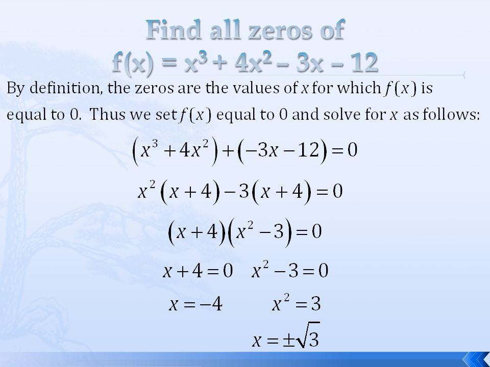
18. IIf f is a polynomial function, then the values of x for which f(x) = 0 are called the zeros of f. TThese values of x are the roots, or solutions (factors), of the polynomial equation f(x) = 0. Each real root of the polynomial equation appears as an x-intercept of the graph of the polynomial function. We usually find these by factoring.

20. Example 5 Find all zeros of f (x) = -x 4 + 4x 3 - 4x 2 Example 6 Find all zeros of f (x) = x 4 – 4x 2

21. Find all zeros of f (x) = 3 (x + 5) (x + 2) 4 Example 7

22. Complete problems 4, 6, 12, 20, 22, 26, 30 on page 330-331

23.  Open a NEW graph document. Graph the equation on your calculator.  Hit Menu and select option 6: Analyze Graph. Select option 1: Zeros.  Use the vertical line to move to the Lower bound of the x-intercept and hit Enter (or click the mouse pad).  Now move it to the Upper bound of the SAME x-intercept and click again. The ZERO should appear on the graph. Repeat for each zero of the function.  What are the zeros of the function?

24.  Grab your calculator.  Now follow the technology tips to find the zeros.  Try Example 8 on your own. Then go back and check your homework from page 331problems 25-31 odds. You have 9 minutes to do all of this.

25. Example 8 Find all zeros of f (x) = x 3 + x 2 + 1 Page 312 Problems 25 – 32 only find the ZEROS

26.  We can use the results of factoring to express a polynomial as a product of factors. For instance, in Example 5, we used our factoring to express the function as follows:  Notice that each factor occurs twice. If the same factor occurs multiple times, we call this a zero with multiplicity of 2.  For the polynomial function f (x), 0 and 2 each have a multiplicity of 2.  Multiplicity means the amount of times a zero repeats itself in the completely factored form.  If the multiplicity is even, the graph “touches” the x-axis.  If the multiplicity is odd, the graph “crosses” the x-axis.

27. Example 9 Find all zeros and multiplicity of Example 10 Find all zeros and multiplicity of

28. Example 11 Find all zeros of f (x) = x 3 + 4x 2 + 4x Example 12 Find all zeros of f (x) = 3 (x + 5) (x + 2) 4 Page 312 Problems 25 – 32 find the zeros and state the Multiplicity

29. Example: Further Explanation Find the zeros of f (x) = (x- 3) 2 (x-1) 3 and give the multiplicity of each zero. State whether the graph crosses the x-axis or touches the x-axis and turns around at each zero. Continued on the next slide.

30. Example: Further Explanation Cont.

31.  The Intermediate Value Theorem tells us of the existence of real zeros. The idea behind the theorem is illustrated in Figure 2.22.  The figure shows that if (a, f (a)) lies below the x-axis and (b, f (b)) lies above the x-axis the smooth, continuous graph of the function must cross the x-axis at some value c between a and b.b.  This value c is a real zero for the function. This also occurs vice versa.

32. Example 13 Show that the polynomial function f (x) = x 3 – 2x + 9 has a real zero between - 3 and - 2.

33. Show that the function y = x 3 – x + 5 has a zero between -2 and -1. Example 14 Page 312 Problems 33 – 40

34. TThe graph of f (x) = x 5 – 6x 3 + 8x + 1 is shown. TThe graph has four smooth turning points. TThe polynomial is of degree 5. Notice that the graph has four turning points. IIn general, if the function is a polynomial function of degree n, then the graph has at most n - 1 turning points. CConversely, if the graph has m amount of turns, the degree of the polynomial is m + 1

35. Example 15 f (x) = x 3 + 4x 2 + 4x Example 16 f (x) = 3 (x + 5) (x + 2) 4

37. Example 17 Graph f (x) = x 4 – 2x2 2x2 + 1. Step 1Determine end behavior (max turning points) Step 2Find zeros Step 3Find y-intercept Step 4Use even/odd symmetry to draw Page 312-313 Problems 41 – 64

38. Example 18 Now graph this function on your calculator. f (x) = (x- 3) 2 (x-1) 3 Step 1 Determine end behavior Step 2 Find zeros Step 3Find y-intercept Step 4Use even/odd symmetry to draw

39. Example Graph f(x) = x 3 – 9x 2 Step 1 Determine end behavior Step 2 Find zeros Step 3Find y-intercept Step 4Use even/odd symmetry to draw

40. Add these problems to your notes paper to help you review! Additional Practice problems can be found on page 313 - 315 problems 65-99

41. (a) (b) (c) (d) Use the Leading Coefficient Test to determine the end behavior of the graph of the polynomial function f(x) = x 3 – 9x 2 + 27 Example 1

42. (a) (b) (c) (d) State whether the graph crosses the x-axis, or touches the x-axis and turns around at the zeros of 1, and - 3. f(x) = (x-1) 2 (x+3) 3 Example 2