Download presentation
Presentation is loading. Please wait.

1
LECTURE NOTE ON Fluid Machines (MCE 513) CREDIT UNIT – 2
BY Dr. Oyedepo, S.O

2
Brief Course Description
This Course provides an in-depth knowledge of the fluid flow in turbo- machineries and positive displacement machines. In addition, the course exposes students to different areas of applications of fluid machines.

3
Course Objectives At the end of this course, the students should be able to: Identify various types of pumps and turbines, and understand how they work Apply dimensional analysis to design new pumps or turbines that are geometrically similar to existing pumps or turbines. Perform basic vector analysis of the flow into and out of pumps and turbines Use specific speed for preliminary design and selection of pumps and turbines Carry out performance analysis on pump, turbine, compressor etc

4
Course Outlines Introduction to fluid machinery
Classification of fluid machines Theory of rotodynamics/Turbo- machines Performance Analysis of fluid machinery Water turbines. The Pelton wheel, Francis turbine. Axial flow turbines. The fluid coupling and the torque converter. Reciprocating Machines

5
References Lakshminarayana, B(1996), Fluid Dynamics and Heat Transfer of Turbomachinery, John Wiley & Sons, Inc. Dixon, S.L (1998), Fluid Mechanics, Thermodynamics of Turbomachinery (5th Ed.) Elsevier Dixon, S.L and Hall, C.A(2010), Fluid Mechanics and Thermodynamics of Turbomachinery (6th Ed.), Elsevier Pritchard, P.J and Leylegian, J.C (2011), Introduction to Fluid Mechanics (8th Ed.), John Wiley & Sons, Inc Douglas, J.F, Gasiorek, J.M, Swaffield, J.A and Jack,L.D (2005),Fluid Mechanics(6th Ed.), Pearson Prentice Hall, USA
, Fluid Mechanics, Thermodynamics of Turbomachinery (5th Ed.) Elsevier. Dixon, S.L and Hall, C.A(2010), Fluid Mechanics and Thermodynamics of Turbomachinery (6th Ed.), Elsevier. Pritchard, P.J and Leylegian, J.C (2011), Introduction to Fluid Mechanics (8th Ed.), John Wiley & Sons, Inc. Douglas, J.F, Gasiorek, J.M, Swaffield, J.A and Jack,L.D (2005),Fluid Mechanics(6th Ed.), Pearson Prentice Hall, USA.")
6
Chapter 1: Introduction and Classification of Fluid Machinery
Fluid machines may be broadly classified as either positive displacement or dynamic. In positive-displacement machines, energy transfer is accomplished by volume changes that occur due to movement of the boundary in which the fluid is confined. This includes piston-cylinder arrangements, gear pumps (for example, the oil pump for a car engine), and lobe pumps (for example, those used in medicine for circulating blood through a machine).
, and lobe pumps (for example, those used in medicine for circulating blood through a machine).")
7
Introduction Contd. Dynamic fluid-handling devices that direct the flow with blades or vanes attached to a rotating member are termed turbomachines. In contrast to positive displacement machinery, there is no closed volume in a turbomachine.

8
Classification of Fluid Machines

9
Classification of Fluid Machines
Based on the classification of fluid machineries, this course is divided into two parts: Turbo- machinery Positive displacement machines

10
Definition of Turbo-Machinery
Turbo-machines are devices in which energy is transferred either to or from a continuously flowing fluid by the dynamic action of one or more moving blade rows. The word turbo is of Latin origin, meaning "that which spins." The rotor changes the stagnation enthalpy, kinetic energy, and stagnation pressure of the fluid. In a compressor or pump, the energy is imparted to the fluid by a rotor. In a turbine, the energy is extracted from the fluid.

11
Turbo-Machinery Contd
Every common turbo-machine contains a rotor upon which blades are mounted, only the detailed physical arrangements differ. Fluid flows through the rotor from an entrance to an exit submit a change in momentum during the process because of the torque exerted on or by rotor blades.

12
Turbo-Machinery Contd.
Turbo-machinery is a major component in (a) aircraft, marine, space (liquid rockets), and land propulsion systems, (b) hydraulic, gas, and steam turbines, (c) industrial pipeline and processing equipment such as gas, petroleum, and water pumping plants, and (d) a wide variety of other applications (e.g., heart-assist pumps, industrial compressors, and refrigeration plants).
 aircraft, marine, space (liquid rockets), and land propulsion systems, (b) hydraulic, gas, and steam turbines, (c) industrial pipeline and processing equipment such as gas, petroleum, and water pumping plants, and. (d) a wide variety of other applications (e.g., heart-assist pumps, industrial compressors, and refrigeration plants).")
13
Turbo-Machinery Contd
A turbo-machinery without a shroud or annulus wall near the tip is termed extended Examples of this are aircraft and ship propellers, wind turbines, etc. On the other hand, enclosed machines are accommodated in a casing so that a finite quantity of fluid passes through the machine per unit of time. Examples of this are jet engine compressors, turbines, and pumps.

14
Classification of Turbo-Machinery

15
Classification of Turbo-Machinery
Two main categories of turbomachine are identified: Firstly, those that absorb power to increase the fluid pressure or head (ducted fans, compressors and pumps); secondly, those that produce power by expanding fluid to a lower pressure or head (hydraulic, steam and gas turbines).
; secondly, those that produce power by expanding fluid to a lower pressure or head (hydraulic, steam and gas turbines).")
16
Classification of Turbo-Machinery Contd
Turbomachines are further categorised according to the nature of the flow path through the passages of the rotor. When the path of the through-flow is wholly or mainly parallel to the axis of rotation, the device is termed an axial flow turbomachine When the path of the through-flow is wholly or mainly in a plane perpendicular to the rotation axis, the device is termed a radial flow turbomachine If the flow path is partially axial and partially radial, the device is called mixed-flow turbomachinery.

17
Classification of Turbo-Machinery Contd
One further category is either impulse or reaction machines according to whether pressure changes are absent or present respectively in the flow through the rotor. In an impulse machine all the pressure change takes place in one or more nozzles, the fluid being directed onto the rotor.

18
Classification of Turbo-Machinery

19
Classification of Turbo-Machinery Contd
Machines for Doing Work on a Fluid Machines that add energy to a fluid by performing work on it are called Pumps when the flow is liquid or slurry, and Fans, blowers, or compressors for gas- or vapour handling units.

20
Classification of Turbo-Machinery Contd
Pumps and compressors consist of a rotating wheel (called an impeller or rotor, depending on the type of machine) driven by an external power source (e.g., a motor or another fluid machine) to increase the flow kinetic energy, followed by an element to decelerate the flow, thereby increasing its pressure. This combination is known as a stage. These elements are contained within a housing or casing. A single pump or compressor might consist of several stages within a single housing, depending on the amount of pressure rise required of the machine
 driven by an external power source (e.g., a motor or another fluid machine) to increase the flow kinetic energy, followed by an element to decelerate the flow, thereby increasing its pressure. This combination is known as a stage. These elements are contained within a housing or casing. A single pump or compressor might consist of several stages within a single housing, depending on the amount of pressure rise required of the machine.")
21
Classification of Turbo-Machinery Contd
Machines for Extracting Work (Power) from a Fluid Machines that extract energy from a fluid in the form of work (or power) are called turbines. In hydraulic turbines, the working fluid is water, so the flow is incompressible. In gas turbines and steam turbines, the density of the working fluid may change significantly. In a turbine, a stage normally consists of an element to accelerate the flow, converting some of its pressure energy to kinetic energy, followed by a rotor, wheel, or runner extracts the kinetic energy from the flow via a set of vanes, blades, or buckets mounted on the wheel.
 from a Fluid. Machines that extract energy from a fluid in the form of work (or power) are called turbines. In hydraulic turbines, the working fluid is water, so the flow is incompressible. In gas turbines and steam turbines, the density of the working fluid may change significantly. In a turbine, a stage normally consists of an element to accelerate the flow, converting some of its pressure energy to kinetic energy, followed by a rotor, wheel, or runner extracts the kinetic energy from the flow via a set of vanes, blades, or buckets mounted on the wheel.")
22
Applications of Turbo machinery
Some typical examples of turbomachinery used in various applications are listed below. Aerospace Vehicle Application. Compressors and turbines are used in gas turbines for power and propulsion of aircraft, helicopters, unmanned aerospace vehicles, V/STOL aircraft, missiles, and so on. Turbines and pumps are used in liquid rocket engines utilized for the propulsion of space vehicles.

23
Applications of Turbo machinery Contd.
Marine Vehicle Application. Turbomachinery components are used in (a) power plants for submarines, hydrofoil boats, Naval surface ships, hovercraft, and so on and (b) propeller and propulsion plants used in ships, underwater vehicles, hydrofoil boats, and so on. Land Vehicle Application. Turbomachinery is an important component in the gas turbines used in trucks, cars, and high- speed train systems. An automotive gas turbine which utilizes a centrifugal compressor and a radial turbine is shown in Fig. below:
 power plants for submarines, hydrofoil boats, Naval surface ships, hovercraft, and so on and (b) propeller and propulsion plants used in ships, underwater vehicles, hydrofoil boats, and so on. Land Vehicle Application. Turbomachinery is an important component in the gas turbines used in trucks, cars, and high- speed train systems. An automotive gas turbine which utilizes a centrifugal compressor and a radial turbine is shown in Fig. below:")
24
Automotive Gas Turbine

25
Applications of Turbo machinery Contd.
Energy Application. Steam turbines are used in steam, nuclear, and coal power plants; hydraulic turbines are used in hydropower plants; gas turbines are used in gas turbine power plants; wind turbines also belong to this class. A large Francis turbine used in hydropower applications is shown in Fig. below.

26
Applications of Turbo machinery Contd.
Industrial Applications. Compressors and pumping machinery are used in gas and petroleum transmissions and other industrial and processing applications; pumping machinery is used in fire fighting, water purification, and pumping plants; high-speed miniature turbo expanders are used in refrigeration equipment; compressors are used in refrigeration plants (industrial and other uses). Miscellaneous. Pumps are used in heart-assist devices, automotive torque converters, swimming pools, and hydraulic brakes. One of the interesting applications of turbo- machinery is in the medical field, the artificial heart pump.
. Miscellaneous. Pumps are used in heart-assist devices, automotive torque converters, swimming pools, and hydraulic brakes. One of the interesting applications of turbo- machinery is in the medical field, the artificial heart pump.")
27
Francis reversible pump-turbine

28
Chapter 2: Basic Governing Equations for Turbo-machines
The Continuity Equation. The Steady Flow Energy Equation (which is in fact a statement of the First Law of Thermodynamics for steady flow systems). Newton's Second Law of Motion. The Second Law of Thermodynamics. The laws of Aerodynamics or Hydrodynamics. Dimensional analysis.
. Newton s Second Law of Motion. The Second Law of Thermodynamics. The laws of Aerodynamics or Hydrodynamics. Dimensional analysis.")
29
Basic Governing Equations for Turbomachines Contd
The basic physical laws (1) to (3) listed above will now be expressed in forms suitable for turbomachinery analysis. We first define a control volume to suit the mixed-flow fan shown in Fig. below. We will define the inlet plane 1-1 and the exit plane 2-2 which have areas A1 and A2 respectively. For simplicity we will assume uniform entry and exit velocities C1 and C2 and also constant densities ρ1 and ρ2 across the planes 1-1 and 2-2.
 to (3) listed above will now be expressed in forms suitable for turbomachinery analysis. We first define a control volume to suit the mixed-flow fan shown in Fig. below. We will define the inlet plane 1-1 and the exit plane 2-2 which have areas A1 and A2 respectively. For simplicity we will assume uniform entry and exit velocities C1 and C2 and. also constant densities ρ1 and ρ2 across the planes 1-1 and 2-2.")
30
Control Volume for a mixed flow fan

31
Continuity Equation Assuming the mass flow rate ṁ= dm/dt through the annulus to be conserved, We may express the principle of mass flow conservation through This is the most simple one-dimensional form of continuity equation, applicable to a system as a whole.

32
Continuity Equation Contd
If we wish to focus instead upon some local infinitesimal region of a system, An equivalent differential form of the above equation may be derived in any selected coordinate system.

33
Continuity Equation in Cartesian Plane
With reference to Fig. below(a), the continuity equation in plane cartesian (x,y) coordinates becomes
, the continuity equation in plane cartesian (x,y) coordinates becomes.")
34
Fluid elements in: (a) (x, y) cartesian coordinates; (b) (x, r) cylindrical coordinates
 (x, y) cartesian coordinates; (b) (x, r) cylindrical coordinates")
35
Continuity Equation in Cylindrical Coordinates
The equivalent compressible flow continuity equation applicable to turbomachinery meridional flows in cylindrical coordinate is

36
Steady flow energy equation
If the First Law of Thermodynamics is applied to the control volume of mixed flow fan we obtain the steady flow energy equation,

37
Momentum equation- Euler pump and Euler turbine equations
Instead of the full control volume of mixed flow fan, we consider next the flow of fluid through the elementary stream tube ψ0 passing through the pump rotor between stations 1 and 2, (See Fig. Below) By applying Newton's second law to the elementary control volume, Fig. (b) below, we have Applied torque = rate of change of moment of momentum
 By applying Newton s second law to the elementary control volume, Fig. (b) below, we have. Applied torque = rate of change of moment of momentum.")
38
(a) Meridional flow through a pump or fan rotor; (b) Stream - tube flowing
 Meridional flow through a pump or fan rotor; (b) Stream - tube flowing")
39
Analytical Expression for Torque

40
Momentum Equation Contd
Making use of the steady flow energy equation and Neglecting the heat transfer rate into the control volume, i.e. Q = 0, We obtain finally the well-known Euler pump equation for fans with compressible fluids:

41
Momentum Equation Contd
For incompressible fluids, i.e. liquids or low Mach number gases, Using the incompressible steady flow energy equation instead, namely

42
Momentum Equation Contd
To obtain the corresponding form of the Euler pump equation, namely

43
Momentum Equation Contd
The Euler pump and turbine equations as derived here are one-dimensional equations in the sense that they are applicable to unit mass of fluid flowing along the line mapped out by the elementary stream tube.

44
Theory of Turbomachines (Rotodynamic Machines):
All rotodynamic machines have a rotating part called the impeller, through which the fluid flow is continuous. The direction of fluid flow in relation to the plane of impeller rotation distinguishes different classes of rotodynamic machines. One possibility is for the flow to be perpendicular to the impeller(as in Fig. (a)below). Machines of this kind are called axial flow machines.
below). Machines of this kind are called axial flow machines.")
45
Theory of Turbomachines Contd
In Centrifugal machines (sometimes called ‘radial flow’), although the fluid approaches the impeller axially, it turns at the machine’s inlet so that the flow through the impeller is in the plane of the impeller rotation (as in Fig. (b) below). Mixed flow machines constitute a third category. They derive their name from the fact that the flow through their impellers is partly axial and partly radial.
, although the fluid approaches the impeller axially, it turns at the machine’s inlet so that the flow through the impeller is in the plane of the impeller rotation (as in Fig. (b) below). Mixed flow machines constitute a third category. They derive their name from the fact that the flow through their impellers is partly axial and partly radial.")
46
Theory of Turbomachines Contd

47
Velocity Triangles The velocity vector of a fluid particle that flows through a turbomachine is most conveniently expressed by its components in cylindrical coordinates. The vector sum of radial and axial components is given by This is called meridional velocity

48
Meridional and tangential components of absolute velocity

49
Velocity Triangles Contd
For axial machines the radial component of velocity is small and can be ignored, making the meridional velocity equal to the axial velocity. Similarly, at the outlet of a centrifugal compressor, or a radial pump, the axial velocity vanishes and the meridional velocity then equals the radial velocity.

50
A typical velocity triangle
Figure (1*)
")
51
Velocity Triangle Contd
The absolute velocity V is the sum of the relative velocity W and the velocity of the frame, or blade velocity U. They are related by the vector equation V= U + W (*) The angle that the absolute velocity makes with the meridional direction is denoted by α, The angle that the relative velocity makes with the relative direction is β. These are called the absolute and relative flow angles.
 The angle that the absolute velocity makes with the meridional direction is denoted by α, The angle that the relative velocity makes with the relative direction is β. These are called the absolute and relative flow angles.")
52
Velocity Triangle Contd
From Eq. (*) and Figure 1* it is seen that the meridional components yield The tangential components are given by These velocities are related to the meridional velocity by and
 and Figure 1* it is seen that the meridional components yield. The tangential components are given by. These velocities are related to the meridional velocity by. and.")
53
Worked Example 1.1 Consider the velocity diagram shown in Figure below. The magnitude of the absolute velocity is V1 = 240m/s, and the flow angle is α = -20°. The blade speed is U = 300 m/s. Find the magnitude of the relative velocity and its flow angle.

55
Solution

56
Chapter 3: One Dimensional Theory
The real flow through an impeller is three dimensional That is to say the velocity of the fluid is a function of three positional coordinates, say, in the cylindrical system, r, θ and z, as shown in Fig. below. Thus, there is a variation of velocity not only along the radius but also across the blade passage in any plane parallel to the impeller rotation Also, there is a variation of velocity in the meridional plane, i.e. along the axis of the impeller. The velocity distribution is therefore, very complex and dependent upon the number of blades, their shapes and thicknesses, as well as on the width of the impeller and its variation with radius.

57
A Centrifugal Impeller in Relation to Cylindrical Coordinates

58
Basic Assumptions The one-dimensional theory simplifies the problem very considerably by making the following assumptions: The blades are infinitely thin and the pressure difference across them is replaced by imaginary body forces acting on the fluid and producing torque. The number of blades is infinitely large, so that the variation of velocity across blade passages is reduced and tends to zero. Thus,

59
Basic Assumptions Contd
there is no variation of velocity in the meridional plane, i.e. across the width of the impeller. Thus, As a result of the above assumptions, the flow through, say, a centrifugal impeller may be represented by a diagram shown in Fig. below.

60
One-dimensional flow through a centrifugal impeller

61
Basic Assumptions Contd
The above assumptions enable us to limit our analysis to changes of conditions which occur between impeller inlet and impeller outlet without reference to the space in between, where the real transfer of energy takes place. This space is treated as a ‘black box’ having an input in the form of an inlet velocity triangle and an output in the form of an outlet velocity triangle. Such velocity triangles for a centrifugal impeller rotating with a constant angular velocity ω are shown in Fig. above.

62
Analysis At inlet, the fluid moving with an absolute velocity v1 enters the impeller through a cylindrical surface of radius r1 and may make an angle α1 with the tangent at that radius. At outlet, the fluid leaves the impeller through a cylindrical surface of radius r2, absolute velocity v2 inclined to the tangent at outlet by the angle α2.

63
Analysis Contd. The velocity triangles shown in Fig. above are obtained as follows. The inlet velocity triangle is constructed by first drawing the vector representing the absolute velocity v1 at an angle α1. The tangential velocity of the impeller, u1 is then subtracted from it vectorially in order to obtain vr1, the relative velocity of the fluid with respect to the impeller blades at the radius r1. In this basic velocity triangle, the absolute velocity v1 is resolved into two components: One in the radial direction, called velocity of flow vf1, and The perpendicular to it i.e in the tangential direction, vw1, sometimes called velocity of whirl. These two components are useful in the analysis and, therefore, they are always shown as part of the velocity triangles.

64
Analysis Contd. From One-dimensional flow through a centrifugal impeller coupled with Newton’s second law applied to angular motion, Torque = Rate of change of angular momentum Now, Angular momentum = (Mass) x (Tangential velocity) x (Radius).
 x (Tangential velocity) x (Radius).")
65
One-dimensional flow through a centrifugal impeller

66
Analysis Contd

67
Analysis Contd

68
Analysis Contd. Equation (1.4) is known as Euler’s equation.
From its mode of derivation it is apparent that Euler’s equation applies to a pump (as derived) and to a turbine. In the case of a turbine, however, since E would be negative, indicating the reversed direction of energy transfer. It is, therefore, common for a turbine to use the reversed order of terms in the brackets to yield positive E. Since the units of E reduce to metres of the fluid handled, it is often referred to as Euler’s head. It is useful to express Euler’s head in terms of the absolute fluid velocities rather than their components. From the velocity triangles of Fig. above,
 and to a turbine. In the case of a turbine, however, since. E would be negative, indicating the reversed direction of energy transfer. It is, therefore, common for a turbine to use the reversed order of terms in the brackets to yield positive E. Since the units of E reduce to metres of the fluid handled, it is often referred to as Euler’s head. It is useful to express Euler’s head in terms of the absolute fluid velocities rather than their components. From the velocity triangles of Fig. above,")
69
Analysis Contd

70
Analysis Contd In the above expression,
The first term denotes the increase of the kinetic energy of the fluid in the impeller. The second term represents the energy used in setting the fluid in a circular motion about the impeller axis (forced vortex). The third term is the regain of static head due to a reduction of relative velocity in the fluid passing through the impeller.
. The third term is the regain of static head due to a reduction of relative velocity in the fluid passing through the impeller.")
71
Application of Euler’s Equation to Centrifugal and Axial Flow Machines
Centrifugal Flow Machine For centrifugal flow machine, the velocity triangles are as shown in Fig. above. In addition, the following relationships hold. In general, u = ωr, it follows that the tangential blade velocities at inlet and outlet are given by

72
Application of Euler’s Equation to Centrifugal Flow Machines Contd.

73
Application of Euler’s Equation to Centrifugal Flow Machines Contd.

74
Centrifugal Flow Machine
At inlet the usual assumptions are as follows:

75
Centrifugal Flow Machine

76
Centrifugal Flow Machine

77
Centrifugal Flow Machine

78
Axial Flow Machine An axial flow machine, is as shown in Fig. below.
In the axial flow machine the flow is axial, the changes from inlet to outlet take place at the same radius.

79
Axial Flow Machine

80
Axial flow impeller and velocity triangles

81
Axial Flow Machine The following assumptions are made with regard to the velocity triangles: 3. At outlet, the relative velocity leaves the blade tangentially and a similar procedure to that for a centrifugal impeller is used to complete the velocity triangles.

82
Axial Flow Machine From the outlet triangle,

83
Axial Flow Machine For any two radii ra and rb,

84
Axial Flow Machine

85
Worked Example 1.2 The shaft of small turbine turns at rpm, and the blade speed is U = 250 m/s. The axial velocity leaving the stator is Vx2 = 175 m/s. The angle at which the absolute velocity leaves the stator blades is α2 = 67°, the flow angle of the relative velocity leaving the rotor is β3= -60°, and the absolute velocity leaves the rotor at the angle α3 = -20°. These are shown in Figure below. Find (a) the mean radius of the blades, (b) the angle of the relative velocity entering the rotor, (c) the magnitude of the axial velocity leaving the rotor, (d) the magnitude of the absolute velocity leaving the stator, and (e) the specific work delivered by the stage.
 the mean radius of the blades, (b) the angle of the relative velocity entering the rotor, (c) the magnitude of the axial velocity leaving the rotor, (d) the magnitude of the absolute velocity leaving the stator, and (e) the specific work delivered by the stage.")
87
Solution In turbines, a stage consists of a stator followed by a rotor
The inlet to the stator is designated as location 1, the inlet to the rotor is location 2, and the exit from the rotor is location 3. The Euler turbine equation is written as w = U2Vu2 - U3Vu3 From Euler equation, the axial component of velocity is denoted as Vx and the component of the velocity in the direction of the blade motion as Vu.

88
Solution Contd For an axial turbomachine U1=U2 = U.
Hence, Work delivered by a stage is then given by w = U(Vu2 - Vu3) (a) The mean radius of the rotor is
 (a) The mean radius of the rotor is.")
90
Trothalpy and specific work in terms of velocities
Rothalpy is a compound word combining the terms rotation and enthalpy. Since no work is done in the turbine stator , total enthalpy remains constant across it. In this section an analogous quantity to the total enthalpy is developed for the rotor.

91
Trothalpy and specific work in terms of velocities Contd
Specifically, consider a mixed-flow compressor in which the meridional velocity at the inlet is not completely axial and at the exit from the blades not completely radial. The work done by the rotor blades is This can be written as

92
Trothalpy and specific work in terms of velocities Contd
The quantity

93
Trothalpy and specific work in terms of velocities Contd

94
Trothalpy and specific work in terms of velocities Contd
This gives

95
Degree of reaction Degree of reaction, or reaction for short, is defined as the change in static enthalpy across the rotor divided by the static enthalpy change across the entire stage. For the turbine this is given as

96
Degree of Reaction Contd
Work delivered by a rotor in a turbine is Since for nozzles (or stator) h01 = h02, work can also be written as
 h01 = h02, work can also be written as.")
97
Degree of Reaction Contd
Solving the last two equations for static enthalpy differences and substituting them into the definition of reaction gives

98
Degree of Reaction Contd
In a flow in which V1 = V2, the reaction R = 1. Such a machine is a pure reaction machine. A lawn sprinkler, rotating about an axis is such a machine, for all the pressure drops take place in the sprinkler arms. They turn as a reaction to the momentum leaving them. In a steam turbine with an axial flow machine in which U2 = U3 its reaction is zero when W2 = W3.

99
Worked Example Consider an axial turbine stage with blade speed U = 350 m/s and axial velocity Vx = m/s. Flow enters the rotor at angle α2 = 60°. It leaves the rotor at angle α3 = -30°. Assume a stage for which α1 = α3 and a constant axial velocity. Find the velocities and the degree of reaction.

100
Solution Since axial velocity is constant and the flow angles are equal at both the entrance and exit of the stage, the velocity diagrams at the inlet of the stator and the exit of the rotor are identical. From a velocity triangle, such as shown in Figure 1.9a, the tangential velocities are:

102
UTILIZATION A measure of how effectively a turbine rotor converts the available kinetic energy at its inlet to work is called utilization, and a utilization factor is defined as the ratio

103
UTILIZATION Contd From equation above, the denominator is the available energy consisting of what is converted to work and the kinetic energy that leaves the turbine. This expression for utilization equals unity if the exit kinetic energy is negligible. But the exit kinetic energy cannot vanish completely because the flow has to leave the turbine. Hence utilization factor is always less than one. Maximum utilization is reached by turning the flow so much that the swirl component vanishes; that is, for the best utilization the exit velocity vector should lie on the meridional plane.

104
UTILIZATION Contd Making the appropriate changes in Eq. (1.22) to make it applicable to a turbine and substituting it into Eq. (1.29), gives an expression for utilization That is in term of velocities alone

105
UTILIZATION Contd From Eq. (1.27) it is easy to see that the work delivered is also
 it is easy to see that the work delivered is also")
106
Utilization Contd In the situation in which R = 1 and therefore also V2 = V1, this expression becomes indeterminate. It is valid for other values of R. In a usual design of a multistage axial turbine the exit velocity triangle is identical to the velocity triangle at the inlet of a stage. Under this condition V1 = V3 and α1 = α3, and the utilization factor simplifies to

107
Utilization Contd

108
Utilization Contd At maximum utilization α3 = 0 and the work is w = UVu2. Equating this to the work given in Eq. (1.35) leads to the equality
 leads to the equality.")
109
Maximum utilization factor
is obtained. For maximum utilization, V3 = Vx3, and solving Eq. (1.33) for this ratio gives
 for this ratio gives.")
110
Maximum utilization factor Contd
If a stage is designed such that Vx3 = Vx2, then the speed ratio in Eq. (1.37) may be written as follows:
 may be written as. follows:")
111
Maximum utilization factor Contd

112
Maximum utilization factor Contd
Inspection of Figure above, as well as Eq. (1.41), shows that maximum utilization factor increases from zero to unity, when the nozzle angle α2 increases from zero to α2 = 90°. Hence large nozzle angles give high utilization factors. Typically the first stage of a steam turbine has R = 0, with a nozzle angle in the range from 65° to 78°.
, shows that maximum utilization factor increases from zero to unity, when the nozzle angle α2 increases from zero to α2 = 90°. Hence large nozzle angles give high utilization factors. Typically the first stage of a steam turbine has R = 0, with a nozzle angle in the range from 65° to 78°.")
113
Worked Example Combustion gases flow from a stator of an axial turbine with absolute speed V2 = 500 m/s at angle α2 = 67°. The relative velocity is at an angle β2 = 30° as it enters the rotor and at β3 = - 65° as it leaves the rotor, (a) Find the utilization factor, and (b) the reaction. Assume the axial velocity to be constant.
 Find the utilization factor, and (b) the reaction. Assume the axial velocity to be constant.")
114
Solution The axial and tangential velocity components at the exit of the nozzle are

115
Since the axial velocity remains constant, at the rotor exit the tangential component of the relative velocity is obtained as:

116
To calculate the utilization factor using its definition Eq. (4
To calculate the utilization factor using its definition Eq. (4.19), work is first determined to be
, work is first determined to be.")
117
Chapter 4: Dimensional Analysis and Similitude of Turbomachines
Dimensional analysis is found to be a very useful tool in fluid flow analysis. In dimensional analysis the number of parameters can be reduced generally to three by grouping relevant variables to form dimensionless parameters. In addition these groups facilitate the presentation of the results of the experiments effectively and also to generalize the results so that these can be applied to similar situations. In dimensional analysis all physical relationships can be reduced to the fundamental quantities of force F, length L, and time T, (and temperature in case of heat).
.")
118
Methods of Determination of Dimensionless Groups
The basic procedures usually used in dimensional analysis are: Intuitive method: This method relies on basic understanding of the phenomenon and then identifying competing quantities like types of forces or lengths etc. and obtaining ratios of similar quantities. Some examples are: Viscous force vs inertia force, viscous force vs gravity force or roughness dimension vs diameter.

119
Methods of Determination of Dimensionless Groups Contd
Rayleigh method: In Rayleigh Method A functional power relation is assumed between the parameters and then the values of indices are solved for to obtain the grouping. For example considering a problem in which the drag force F on a stationary sphere in flow is found to depend on diameter D, velocity u, fluid density ρ and viscosity μ. To obtain a curve F vs u, for fixed values of ρ, μ and D one can write The values of a, b, c, d, and e are obtained by comparing the dimensions on both sides. The dimensions on the L.H.S. being zero as π terms are dimensionless.

120
Methods of Determination of Dimensionless Groups Contd
Buckingham Pi theorem method One important procedure usually used in dimensional analysis is the Buckingham π theorem. The statement of the theorem is as follows: If a relation among n parameters exists in the form f (q1, q2, qn) = (1)
 = 0 (1)")
121
Buckingham Pi theorem method Contd
Equation (1)above implies that the n parameters can be grouped into n – m independent dimensionless ratios or π parameters, expressed in the form or where m is the number of dimensions required to specify the dimensions of all the parameters, q1, q2, .... qn.
above implies that the n parameters can be grouped into n – m independent dimensionless ratios or π parameters, expressed in the form. or. where m is the number of dimensions required to specify the dimensions of all the parameters, q1, q2, .... qn.")
122
Determination of π Groups
Step1. List all the parameters that influence the phenomenon concerned. Usually three type of parameters may be identified in fluid flow namely fluid properties, geometry and flow parameters like velocity and pressure. Step2. Select a set of primary dimensions, (mass, length and time), (force, length and time), (mass, length, time and temperature) are some of the sets used popularly.
, (force, length and time), (mass, length, time and temperature) are some of the sets used popularly.")
123
Determination of π Groups Contd
Step3. List the dimensions of all parameters in terms of the chosen set of primary dimensions. Table below Lists the dimensions of various parameters involved.

124
Units and Dimensions of Variables

125
Determination of π Groups Contd
Step 4. Select from the list of parameters a set of repeating parameters equal to the number of primary dimensions. Some guidelines are necessary for the choice. (i) the chosen set should contain all the dimensions (ii) two parameters with same dimensions should not be chosen. Say L, L2, L3, (iii) the dependent parameter to be determined should not be chosen.
 the chosen set should contain all the dimensions. (ii) two parameters with same dimensions should not be chosen. Say L, L2, L3, (iii) the dependent parameter to be determined should not be chosen.")
126
Determination of π Groups Contd
Step 5. Set up a dimensional equation with the repeating set and one of the remaining parameters, in turn to obtain n – m such equations To determine π terms numbering n – m. The form of the equation is, The solution of these set of equations will give the values of a, b, c and d. Thus the π term will be defined.

127
Determination of π Groups Contd
Step 6. Check whether π terms obtained are dimensionless. This step is essential before proceeding with experiments to determine the functional relationship between the π terms. Note: If the number of fundamental dimensions is k, the number of terms will be equal to (n-k). The first π term can be expressed as the product of the chosen quantities each to an unknown exponent and the other quantity to a known power (usually taken as one). For each term, solve for the unknown exponent by dimensional analysis. Any term can be replaced by any power of that term π1 by π12, or by 1/π1, also any term can be multiplied by a numerical constant.
. The first π term can be expressed as the product of the chosen quantities each to an unknown exponent and the other quantity to a known power (usually taken as one). For each term, solve for the unknown exponent by dimensional analysis. Any term can be replaced by any power of that term π1 by π12, or by 1/π1, also any term can be multiplied by a numerical constant.")
128
Determination of π Groups Contd
If we want to find the force on a propeller blade we must first decide what might influence this force. It would be reasonable to assume that the force, F, depends on the following physical properties: d - diameter, u - forward velocity of the propeller (velocity of the plane), ρ - fluid density, N -revolutions per second, μ - fluid viscosity Before we do any analysis we can write this equation: F = f ( d, u, ρ , N, μ) or 0 = f1 ( F, d, u, ρ , N, μ ) where and f and f1 are unknown functions.
, ρ - fluid density, N -revolutions per second, μ - fluid viscosity. Before we do any analysis we can write this equation: F = f ( d, u, ρ , N, μ) or. 0 = f1 ( F, d, u, ρ , N, μ ) where and f and f1 are unknown functions.")
129
Determination of π Groups Contd
These can be expanded into an infinite series which can itself be reduced to F = K dm up dm up ρq Nr μs where K is some constant and m, p, q, r, s are unknown constant powers. From dimensional analysis we 1. obtain these powers 2. form the variables into several dimensionless groups The value of K or the functions and 1 must be determined from experiment. The knowledge of the dimensionless groups often helps in deciding what experimental measurements should be taken.

134
Worked Example The pressure drop ΔP per unit length in flow through a smooth circular pipe is found to depend on (i) the flow velocity, u (ii) diameter of the pipe, D (iii) density of the fluid ρ, and (iv) the dynamic viscosity μ. (a) Using π theorem method, evaluate the dimensionless parameters for the flow. (b) Using Rayleigh method (power index) evaluate the dimensionless parameters.
 the flow velocity, u (ii) diameter of the pipe, D (iii) density of the fluid ρ, and (iv) the dynamic viscosity μ. (a) Using π theorem method, evaluate the dimensionless parameters for the flow. (b) Using Rayleigh method (power index) evaluate the dimensionless parameters.")
135
Solution Choosing the set mass, time and length as primary dimensions, the dimensions of the parameters are tabulated.

136
There are five parameters and three dimensions
There are five parameters and three dimensions. Hence two π terms can be obtained. As ΔP is the dependent variable D, ρ and u are chosen as repeating variables.

137
This term may be recognised as inverse of Reynolds number
This term may be recognised as inverse of Reynolds number. So π2 can be modified as π2 = uρD/μ also π2 = (uD/v). The significance of this π term is that it is the ratio of inertia force to viscous force.
. The significance of this π term is that it is the ratio of inertia force to viscous force.")
138
In case D, u and μ had been chosen as the repeating variables, π1 = ΔPD2/u μ
and π2 = ρDu/μ. The parameter π1/π2 will give the dimensionless term ΔP D/ρU2 In this case π1 represents the ratio pressure force/viscous force. This flow phenomenon is influenced by the three forces namely pressure force, viscous force and inertia force.

139
Rayleigh method(a.k.a method of Indices)
The following functional relationship is formed first. There can be two p terms as there are five variables and three dimensions ∆PaDbρcμdue = (p1 p2), Substituting dimensions,
, Substituting dimensions,")
140
Rayleigh method Contd There are five unknowns and three equations.
Hence some assumptions are necessary based on the nature of the phenomenon. As ∆P, the dependent variable can be considered to appear only once. We can assume a = 1. Similarly, studying the forces, μ appears only in the viscous force. So we can assume d = 1. Solving a = 1, d = 1, b = 0, c = – 2, e = – 3, (p1 p2) = ∆Pμ/ρ2 u3. Multiply and divide by D, then p1 = ∆P D/ρU2 and p2 = μ/ρuD. Same as was obtained by pi theorem method. This method requires more expertise and understanding of the basics of the phenomenon.
 = ∆Pμ/ρ2 u3. Multiply and divide by D, then p1 = ∆P D/ρU2 and p2 = μ/ρuD. Same as was obtained by pi theorem method. This method requires more expertise and understanding of the basics of the phenomenon.")
141
Important Dimensionless Parameters

142
Chapter 5: Application of Dimensional Analysis on Turbomachines:
Consider a series of geometrically similar pumps or turbines of different sizes but having similar flow patterns. The energy transferred E is a function of wheel diameter D, volumetric discharge Qv , fluid density ρ, kinematic viscosity ν and the rotating speed N. These variables could be organized in mathematical form as following:

143
Application of Dimensional Analysis on Turbomachines Contd
where E represents pressure energy = ρ g Ho Following π theorem, we have (6-3) = 3 π terms. Select three independent variables, D, N, E
 = 3 π terms. Select three independent variables, D, N, E.")
144
Application of Dimensional Analysis on Turbomachines Contd

145
Application of Dimensional Analysis on Turbomachines Contd

146
Worked Example The power developed by hydraulic machines is found to depend on the head h, flow rate Q, density ρ, speed N, runner diameter D, and acceleration due to gravity, g. Obtain suitable dimensionless parameters to correlate experimental results.

147
Solution The parameters with dimensions are listed below adopting MLT set of dimensions.

148
Solution Contd Taking ρ, D and g as repeating variables

149
Coefficients in Model Testing
The coefficients popularly used in model testing are given below. These can be obtained from the above four π terms.

150
Discussion of Dimensional Analysis on Turbomachines

151
Similitude and Model Testing
Fluid flow analysis is involved in the design of aircrafts, ships, submarines, turbines, pumps, harbours and tall buildings and structures. Fluid flow is influenced by several factors and because of this the analysis is more complex. For many practical situations exact solutions are not available. The estimates may vary by as much as 20%. Because of this it is not possible to rely solely on design calculations and performance predictions.

152
Similitude and Model Testing Contd
Experimental validation of the design is thus found necessary. Constructing and testing small versions of the unit is called model testing. Similarity of features enables the prediction of the performance of the full size unit from the test results of the smaller unit. The application of dimensional analysis is helpful in planning of the experiments as well as prediction of the performance of the larger unit from the test results of the model.

153
Model and Prototype In the engineering point of view model can be defined as the representation of physical system that may be used to predict the behaviour of the system in the desired aspect. The system whose behaviour is to be predicted by the model is called the prototype. As models are generally smaller than the prototype, these are cheaper to build and test. Model testing is also used for evaluating proposed modifications to existing systems. The effect of the changes on the performance of the system can be predicted by model testing before attempting the modifications. Models should be carefully designed for reliable prediction of the prototype performance.

154
Conditions for Similarity between Models and Prototype
Dimensional analysis provides a good basis for laying down the conditions for similarity. If a model is to be similar to the prototype and also function similarly as the prototype, then the PI terms for the model should also have the same value as that of the prototype or the same functional relationship as the prototype.

155
Conditions for Similarity between Models and Prototype Contd
Performance of any system (prototype) is given by functional relationship: π1p = f (π2p , π3p πnp) The functional relationship as a model is: πlm = f (π2m, π3m πnm) Similarity requirements or modelling laws is given by: πlm = πlp, π2m = π2p, πnm = πnp
 is given by functional relationship: π1p = f (π2p , π3p πnp) The functional relationship as a model is: πlm = f (π2m, π3m πnm) Similarity requirements or modelling laws is given by: πlm = πlp, π2m = π2p, πnm = πnp.")
156
Hydraulic Similarity The main types of hydraulic similitude are:
a) Geometric Similitude (Similarity) The geometric similitude exists between model and prototype if the ratios of corresponding dimensions are equal i.e
 Geometric Similitude (Similarity) The geometric similitude exists between model and prototype if the ratios of corresponding dimensions are equal i.e.")
157
Hydraulic Similarity Contd
b) Dynamic Similitude The dynamic similitude exists between the model and the prototype if both of them have identical forces i.e
 Dynamic Similitude. The dynamic similitude exists between the model and the prototype if both of them have identical forces i.e.")
158
Hydraulic Similarity Contd
c) Kinematic Similitude The kinematic similitude exists between model and prototype when the ratios of the corresponding velocities and acceleration at corresponding points are equal i.e
 Kinematic Similitude. The kinematic similitude exists between model and prototype when the ratios of the corresponding velocities and acceleration at corresponding points are equal i.e.")
159
Types of Model Studies Model testing can be broadly classified on the basis of the general nature of flow into four types. These are Flow through closed conduits Flow around immersed bodies Flow with free surface and Flow through turbomachinery

160
Types of Model Studies Contd
Flow through Closed Conduits Flow through pipes, valves, fittings and measuring devices are dealt under this category. From dimensional analysis the pressure drop in the prototype is calculated as As ΔPm is measured, using the model, the pressure drop in the prototype can be predicted.

161
Types of Model Studies Contd
Flow around Immersed Bodies Aircraft, Submarine, cars and trucks and recently buildings are examples for this type of study. In the sports arena golf and tennis balls are examples for this type of study. Models are usually tested in wind tunnels.

162
Flow around Immersed Bodies
Using the similitude, measured values of drag on model is used to estimate the drag on the prototype.

163
Flow around Immersed Bodies
Flow with Free Surface Flow in canals, rivers as well as flow around ships come under this category. In these cases gravity and inertia forces are found to be governing the situation and hence Froude number becomes the main similarity parameter.

164
Flow with Free Surface Considering Froude number, the velocity of the model is calculated as below.

165
Types of Model Studies Contd
Flow through Turbomachinery Pumps as well as turbines are included in the general term turbomachines. As earlier discussed Pumps are power absorbing machines which increase the head of the fluid passing though them. Turbines are power generating machines which reduce the head of the fluid passing through them.

166
Flow through Turbomachinery
The operating variables of the machines are the flow rate Q, the power P and the speed N. The fluid properties are the density and viscosity. The machine parameters are the diameter and a characteristic length and the roughness of the flow surface.

167
Flow through Turbomachinery Contd
Power, head and efficiency can be expressed as functions of π terms as The dimensionless term involving power is defined as Power coefficient, defined as Cp = P/ρ N3 D3 The head coefficient is defined as Ch = gh/N2D2. The term Q/ND3 is called flow coefficient.

168
Flow through Turbomachinery Contd
If two similar machines are operated with the same flow coefficient, the power and head coefficients will also be equal for the machines. This will then lead to the same efficiency. Combining flow and head coefficients in the case of pumps will give the dimensionless specific speed of the pump i.e

169
Flow through Turbomachinery Contd

170
Worked Example A fan when tested at ground level with air density of 1.3 kg/m3, running at 990 rpm was found to deliver 1.41m3/s at a pressure of 141 N/m2. This is to work at a place where the air density is kg/m3, the speed being 1400 rpm. Determine the volume delivered and the pressure rise.

171
Solution For similarity condition the flow coefficient Q/ND3 should be equal. As D is the same,

172
Worked Example A centrifugal pump with dimensional specific speed (SI) of 2300 running at 1170 rpm delivers 70m3/hr. The impeller diameter is 0.2 m. Determine the flow, head and power if the pump runs at 1750 rpm. Also calculate the specific speed at this condition.
 of 2300 running at 1170 rpm delivers 70m3/hr. The impeller diameter is 0.2 m. Determine the flow, head and power if the pump runs at 1750 rpm. Also calculate the specific speed at this condition.")
173
Solution The head developed and the power at test conditions are determined first (At 1170 rpm).
.")
174
Chapter 6: Pumps Three types of pumps are in use.
Rotodynamic pumps which move the fluid by dynamic action of imparting momentum to the fluid using mechanical energy. Reciprocating pumps which first trap the liquid in a cylinder by suction and then push the liquid against pressure. Rotary positive displacement pumps which also trap the liquid in a volume and push the same out against pressure.

175
Pumps Classification Reciprocating pumps are limited by the low speed of operation required and small volumes it can handle. Rotary positive displacement pumps are limited by lower pressures of operation and small volumes these can handle. Gear, vane and lobe pumps are of this type. Rotodynamic pumps i.e. centrifugal and axial flow pumps can be operated at high speeds often directly coupled to electric motors. These can handle from small volumes to very large volumes. These pumps can handle corrosive and viscous, fluids and even slurries. The overall efficiency is high in the case of these pumps. Hence these are found to be the most popular pumps in use.

176
Rotodynamic pumps Rotodynamic pumps can be of radial flow,
mixed flow and axial flow types according to the flow direction. Radial flow or purely centrifugal pumps generally handle lower volumes at higher pressures. Mixed flow pumps handle comparatively larger volumes at medium range of pressures. Axial flow pumps can handle very large volumes, but the pressure against which these pumps operate is limited. The overall efficiency of the three types are nearly the same.

177
CENTRIFUGAL PUMPS Centrifugal pumps are radial-flow machines that operate most efficiently for applications requiring high heads at relatively low flow rates. These are so called because energy is imparted to the fluid by centrifugal action of moving blades from the inner radius to the outer radius. The main components of centrifugal pumps are (1) the impeller, (2) the casing and (3) the drive shaft with gland and packing.
 the impeller, (2) the casing and (3) the drive shaft with gland and packing.")
178
Centrifugal Pump Contd

179
Classification of Centrifugal Pump
Centrifugal pumps may be classified in several ways. On the basis of speed as low speed, medium speed and high speed pumps. On the basis of direction of flow of fluid, the classification is radial flow, mixed flow and radial flow. On the basis of head pumps may be classified as low head (10 m and below), medium head (10-50 m) and high head pumps. Single entry type and double entry type is another classification. Double entry pumps have blades on both sides of the impeller disc. Figure below illustrates the same.
, medium head (10-50 m) and high head pumps. Single entry type and double entry type is another classification. Double entry pumps have blades on both sides of the impeller disc. Figure below illustrates the same.")
180
Classification of Centrifugal Pump Contd
Single and double entry pumps

181
Classification of Centrifugal Pump Contd
The classification may also be based on the specific speed of the pump. The expression for the dimensionless specific speed is given in equation below.

182
Classification of Centrifugal Pump Contd
Specific Speed Classification of Pumps

183
Pressure Developed by the Impeller
The general arrangement of a centrifugal pump system is shown in Figure below.

184
Pressure Developed by the Impeller Contd
where He is the effective head.

185
Energy Transfer by Impeller
The energy transfer is given by Euler equation applied to work absorbing machines, This can be expressed as ideal head imparted as

186
Energy Transfer by Impeller Contd
The velocity diagrams at inlet and outlet of a backward curved vaned impeller is shown in figure below. The inlet whirl is generally zero. There is no guide vane at inlet to impart whirl. So the inlet triangle is right angled.

187
Energy Transfer by Impeller Contd

188
Energy Transfer by Impeller Contd
Manometric efficiency is defined as the ratio of manometric head and ideal head

189
Losses in Centrifugal Pumps
(i) Mechanical friction losses between the fixed and rotating parts in the bearings and gland and packing. (ii) Disc friction loss between the impeller surfaces and the fluid. (iii) Leakage and recirculation losses. The recirculation is along the clearance between the impeller and the casing due to the pressure difference between the hub and tip of the impeller.
 Mechanical friction losses between the fixed and rotating parts in the bearings and gland and packing. (ii) Disc friction loss between the impeller surfaces and the fluid. (iii) Leakage and recirculation losses. The recirculation is along the clearance between the impeller and the casing due to the pressure difference between the hub and tip of the impeller.")
190
Pump Characteristics We have seen that the theoretical head

191
Pump Characteristics Contd
The characteristic of a centrifugal pump at constant speed is shown in Figure below. It may be noted that the power increases and decreases after the rated capacity. In this way the pump is self limiting in power and the choice of the motor is made easy. The distance between the brake power and water power curves gives the losses.

192
Pump Characteristics Contd
Centrifugal pump characteristics at constant speed

193
Cavitation in Hydraulic Machines
Whenever the pressure in the liquid is reduced to its vapour pressure, the liquid will then boil at that point and bubbles of vapour will form. As the fluid flows into a region of higher pressure the bubbles of vapour will suddenly condense or collapse. This action produces very high dynamic pressure upon the adjacent solid walls and since the action is continuous and has a high frequency the material in that zone will be damaged. Turbine runners and pump impellers are often severely damaged by such action. The process is called cavitation and the damage is called cavitation damage. In order to avoid cavitation, the absolute pressure at all points should be above the vapour pressure.

194
Effects of Cavitation Cavitation causes damage to the runner,
Cavitation results in undesirable vibration noise It leads to loss of efficiency. The flow will be disturbed from the design conditions.

195
AXIAL FLOW PUMP The flow in these machines is purely axial and axial velocity is constant at all radii. The blade velocity varies with radius and so the velocity diagrams and blade angles will be different at different radii. Twisted blade or airfoil sections are used for the blading. Guide vanes are situated behind the impeller to direct the flow axially without whirl. In large pumps inlet guide vanes may also be used. Such pumps are also called as propeller pumps. The head developed per stage is small, but due to increased flow area, large volumes can be handled.

196
AXIAL FLOW PUMP Contd

197
AXIAL FLOW PUMP Contd Comparative values of parameter for different types of pumps

198
Chapter 7: POWER TRANSMITTING SYSTEMS
INTRODUCTION Ordinarily power is transmitted by mechanical means like gear drive or belt drive. In the case of gear drive there is a rigid connection between the driving and driven shafts. The shocks and vibrations are passed on from one side to the other which is not desirable. Also gear drives cannot provide a step-less variation of speeds.

199
Introduction Contd. In certain cases where the driven machine has a large inertia, the driving prime mover like electric motor will not be able to provide a large starting torque. Instead of the mechanical connection if fluids can be used for such drives, high inertia can be met. Also shock loads and vibration will not be passed on. Smooth speed variation is also possible. The power transmitting systems offer these advantages.

200
Types of power transmitting devices
There are two types of power transmitting devices. These are Fluid coupling and Torque converter or torque multiplier.

201
Fluid coupling In this device the driving and driven shafts are not rigidly connected. The drive shaft carries a pump with radial vanes and the driven shaft carries a turbine runner. Both of these are enclosed in a casing filled with oil of suitable viscosity. The pump accelerates the oil by imparting energy to it. The oil is directed suitably to hit the turbine vanes where the energy is absorbed and the oil is decelerated.

202
Fluid Coupling Contd. The decelerated oil now enters the pump and the cycle is repeated. There is no flow of fluid to or from the outside. The oil transfers the energy from the drive shaft to the driven shaft. As there is no mechanical connection between the shafts, shock loads or vibration will not be passed on from one to the other. The turbine will start rotating only after a certain level of energy picked up by the oil from the pump.

203
Fluid coupling Contd Fluid coupling

204
Torque Converter In the case of fluid coupling the torque on the driver and driven members are equal. The application is for direct drives of machines. There are cases where the torque required at the driven member should be more than the torque on the driver. Of course the speeds in this case will be in the reverse ratio. Such an application is in automobiles where this is achieved in steps by varying the gear ratios. The desirable characteristic is a step-less variation of torque.

205
Torque Converter Contd.
The torque converter is thus superior to the gear train with few gear ratios. A sectional view of torque converter is shown in figure below. Torque converter consists of three elements namely pump impeller, a turbine runner and a fixed guide wheel as shown in figure below. The pump is connected to the drive shaft. The guide vanes are fixed. The turbine runner is connected to the driven shaft. All the three are enclosed in a casing filled with oil. The oil passing through the pump impeller receives energy.

206
Torque Converter Contd

207
Worked Example 3.1 The following details refer to a centrifugal pump. Outer diameter: 30 cm. Eye diameter: 15 cm. Blade angle at inlet: 30°. Blade angle at outlet: 25°, Speed rpm. The flow velocity remains constant. The whirl at inlet is zero. Determine the work done per kg. If the manometric efficiency is 82%, determine the working head. If width at outlet is 2 cm, determine the power given that ηo = 76%.

208
Solution

209
Tutorial It is proposed to design a homologous model for a centrifugal pump. The prototype pump is to run at 600 rpm and develop 30 m head the flow rate being 1 m3/s. The model of 1/4 scale is to run at rpm. Determine the head developed discharge and power required for the model. Overall efficiency = 80%.

210
Solution In this case the speeds and diameter ratios are specified.

211
Solution Contd

212
TUTORIAL QUESTIONS At higher speeds where compressibility effects are to be taken into account the performance of a propeller in terms of force exerted is influenced by the diameter, forward speed, rotational speed, density, viscosity and bulk modulus of the fluid. Evaluate the dimensionless parameters for the system.

213
Solution There are seven variables and three dimensions, so four π terms are possible. Selecting D, u and ρ as repeating parameters, The influencing parameters and dimensions are tabulated below, using M, L, T set.

217
Question 2

218
Solution

221
Chapter 8: Reciprocating Machines (or Positive Displacement Machines)
INTRODUCTION In positive displacement machines fluid is drawn into a finite space bounded by mechanical parts, then sealed in it, and then forced out from space and the cycle is repeated. The flow is intermittent and depends on the dimensions of the space (chamber), and speed of the pump.
, and speed of the pump.")
222
Introduction Contd In this chapter we shall describe briefly positive displacement pumps which includes pumps using oil as working fluid. Typical positive displacement pumps: (a) tire pump, (b) human heart, (c) gear pump (d) vane pump
 tire pump, (b) human heart, (c) gear pump (d) vane pump.")
223
Reciprocating Pumps (Positive Displacement Pumps)
There are two main types of pumps namely: the dynamic and positive displacement pumps. Dynamic pumps consist of centrifugal, axial and mixed flow pumps. Positive displacement pumps consist of reciprocating and rotary types. In these types a certain volume of fluid is taken in an enclosed volume and then it is forced out against pressure to the required application.

224
TYPES OF POSITIVE DISPLACEMENT PUMP
The positive displacement pump designs are as follows: (a) Reciprocating type Piston or Plunger type Diaphragm type. (b) Rotary Single rotor such as sliding vane. Multiple rotors such as gear, lobe, and screw type.
 Reciprocating type. Piston or Plunger type. Diaphragm type. (b) Rotary. Single rotor such as sliding vane. Multiple rotors such as gear, lobe, and screw type.")
225
ROTARY PUMPS In Rotary pumps, movement of liquid is achieved by mechanical displacement of liquid produced by rotation of a sealed arrangement of intermeshing rotating parts within the pump casing. One major example of Rotary pump is Gear pump.

226
The Gear Pump In this pump, intermeshing gears or rotors, rotate in opposite directions, just like the gears in a vehicle or a watch mechanism. The pump rotors are housed in the casing or stator with a very small clearance between them and the casing. The fluid being pumped will lubricate this small clearance and help prevent friction and therefore wear of the rotors and casing Figures below show gear pump.

227
The Gear Pump Contd

228
Rotary Pump Contd Rotary pumps are widely used for viscous liquids and are self-lubricating by the fluid being pumped. This means that an external source of lubrication cannot be used as it would contaminate the fluid being pumped. However, if a rotary pump is used for dirty liquids or slurries, solid particles can get between the small clearances and cause wear of the teeth and casing. This will result in loss of efficiency and expensive repair or replacement of the pump.

229
RECIPROCATING PUMPS In a reciprocating pump, a volume of liquid is drawn into the cylinder through the suction valve on the intake stroke and is discharged under positive pressure through the outlet valves on the discharge stroke. The discharge from a reciprocating pump is pulsating and changes only when the speed of the pump is changed. This is because the intake is always a constant volume. Reciprocating pumps are often used for sludge and slurry.

230
RECIPROCATING PUMPS Contd
A reciprocating pump essentially consists of a piston moving to and fro in a cylinder. The piston is driven by a crank powered by some prime mover such an electric motor, IC engine or steam engine.

231
RECIPROCATING PUMPS Contd
In reciprocating pump, when the piston moves to the right as shown in Fig. below the pressure is reduced in the cylinder. This enables water in the lower reservoir to force the liquid up the suction pipe into the cylinder. The suction valve operates only during suction stroke. It is then followed by delivery stroke during which liquid in the cylinder is pushed out through the delivery valve and into the upper reservoir. During the delivery stroke suction valve is closed due to higher pressure. The whole cycle is repeated at a frequency depending upon the rotational speed of the crank.

232
Reciprocating pump installation.

233
Analysis of Reciprocating Pump
Power Output The power output of any pump is the available power to force the liquid to move. The equation of power can be delivered from the following equations by applying Bernoulli’s equation, neglecting hydraulic losses.

234
Analysis of Reciprocating Pump Contd
Shaft Power = Tω

235
Pump Efficiency The internal head, Hi, generated by the pump is greater than pump head, the difference accounting for the internal losses within the pump, hp. Thus,

236
Pump Efficiency Contd If the power input to the pump from the prime mover is Po then overall efficiency set is calculated as follows

237
Pump Efficiency Contd

238
Flow Rate in Single Acting and Double Acting Pump

239
Flow Rate in Single Acting and Double Acting Pump Contd
Slip There can be leakage along the valves, piston rings, gland and packing which will reduce the discharge to some extent. This is accounted for by the term slip.

240
Flow Rate in Single Acting and Double Acting Pump Contd
It has been found in some cases that Qac > Qth, due to operating conditions. In this case the slip is called negative slip. Theoretical power is given by:

241
Worked Example A single acting reciprocating water pump of mm bore and 240 mm stroke operates at 40 rpm. Determine the discharge if the slip is 8%. What is the value of coefficient of discharge? If the suction and delivery heads are 6 m and 20 m respectively determine the theoretical power. If the overall efficiency was 80%, what is the power requirement?

242
Solution

243
HYDRAULIC TURBINE Machines that extract energy from fluid stream are called turbines. They are classified as: Hydraulic turbines (Pelton, Francis, Kaplan) Steam turbines Gas turbines In hydraulic turbines the working fluid is water and is incompressible. More general classification of hydraulic turbines are: impulse reaction
 Steam turbines. Gas turbines. In hydraulic turbines the working fluid is water and is incompressible. More general classification of hydraulic turbines are: impulse. reaction.")
244
Impulse Turbine In the case of impulse turbine all the potential energy is converted to kinetic energy in the nozzles. The impulse provided by the jets is used to turn the turbine wheel. The pressure inside the turbine is atmospheric. This type is found suitable when the available potential energy is high and the flow available is comparatively low. Impulse turbines are driven by one or two high velocity jets. Each jet is accelerated in a nozzle external to the turbine wheel known as turbine rotor. If friction and gravity are neglected the fluid pressure and relative velocity do not change as it passes over the blades/buckets.

245
Reaction Turbine In reaction turbines, the available potential energy is progressively converted in the turbines rotors and the reaction of the accelerating water causes the turning of the wheel. These are again divided into radial flow, mixed flow and axial flow machines. Radial flow machines are found suitable for moderate levels of potential energy and medium quantities of flow. The axial machines are suitable for low levels of potential energy and large flow rates. The potential energy available is generally denoted as “head available”. With this terminology plants are designated as “high head”, “medium head” and “low head” plants.

246
Hydraulic Turbine Terminologies
Head Head is the difference in elevation between two levels of water. The head of a hydroelectric power plant is entirely dependent on the topographical conditions. Head can be characterized as: gross head, and net or effective head. Gross head Is defined as the difference in elevation between the head race level at the intake and the tail race level at the discharge side, naturally, both the elevations have to be measured simultaneously.

247
Hydraulic Turbine Terminologies Contd
Net or effective head Is the head obtained by subtracting from gross head all losses in carrying water from the head race to the entrance of the turbine. The losses are due to friction occurring in tunnels, canals and penstocks which lead the water into the turbine. Net or effective head is, therefore, the true pressure difference between the entrance to the turbine casing and the tail race water elevatio

248
Hydraulic Turbine Terminologies Contd
Flow rate or discharge of water It is the quantities of water used by the water turbine in unit time and is generally measured in (m3/s) or (l/s).
 or (l/s).")
249
Pelton Wheel Turbine The Pelton wheel turbine is a pure impulse turbine in which a jet of fluid leaving the nozzle strikes the buckets fixed to the periphery of a rotating wheel. The energy available at the inlet of the turbine is only kinetic energy. The pressure at the inlet and outlet of the turbine is atmospheric. The turbine is used for high heads ranging from ( ) m. The turbine is named after L. A. Pelton, an American engineer. Pelton wheel is shown in Fig. below.
 m. The turbine is named after L. A. Pelton, an American engineer. Pelton wheel is shown in Fig. below.")
250
Impulse turbine (Pelton wheel)
")
251
Parts of the Pelton turbine
Nozzle and flow control arrangement The nozzle converts the total head at the inlet of the nozzle into kinetic energy. The amount of water striking the curved buckets of the runner is controlled by providing a spear in the nozzle. Runner and buckets The rotating wheel or circular disc is called the runner. On the periphery of the runner a number of buckets evenly spaced are fixed. The buckets deflect the jet through an angle between (160o - 165o) in the same plane as the jet. Due to this deflection of the jet, the momentum of the fluid is changed reacting on the buckets. A bucket is therefore, pushed away by the jet.
 in the same plane as the jet. Due to this deflection of the jet, the momentum of the fluid is changed reacting on the buckets. A bucket is therefore, pushed away by the jet.")
252
Parts of the Pelton turbine Contd
Casing The casing prevents the splashing of the water and discharges the water to tail race.. The casing is made of cast iron or fabricated steel plates. Breaking jet To stop the runner within a short time, a small nozzle is provided which directs the jet of water on to the back of the vanes. The jet of water is called the "breaking jet ". If there is no breaking jet, the runner due to inertia goes on revolving for a long time.

253
Single jet, horizontal shaft pelton turbine

254
Francis Turbine (Reaction Turbine)
Francis turbine is a reaction turbine shown in Fig. below. Water enters circumferentially through turbine casing. It enters from the outer periphery of guide vanes and flows into runner. It flows down the rotor radially and leaves axially. Water leaving the runner flows through a diffuser known as draft tube before entering the tail race.

255
Francis Turbine (Reaction Turbine) Contd
 Contd")
256
Kaplan Turbine (Reaction Turbine)
Kaplan turbine is a reaction turbine shown in Fig. below. The water from the spiral casing enters guide blades similar to Francis. The Kaplan turbine consists of an axial flow runner with 4 to 6 blades of an airfoil section. In this turbine both guide vanes and moving blades are adjustable and therefore high efficiency can be obtained.

257
Kaplan Turbine (Reaction Turbine) Contd
 Contd")
258
Main components of Francis turbine/Kaplan Turbine
Penstock Penstock is a waterway to carry water from the reservoir to the turbine casing. Trashracks are provided at the inlet of penstock in order to obstruct the debris entering in it. Casing The water from penstocks enter the casing which is of spiral shape. In order to distribute the water around the guide ring evenly, the area of cross section of the casing goes on decreasing gradually. The casing is usually made of concrete, cast steel or plate steel.

259
Main components of Francis turbine/Kaplan Turbine Contd
Guide vanes The stationary guide vanes are fixed on stationary circular wheel which surrounds the runner. The guide vanes allow the water to strike the vanes fixed on the runner without shock at the inlet. This fixed guide vanes are followed by adjustable guide vanes. Runner It is circular wheel on which a series of radial curved vanes are fixed. The water passes into the rotor where it moves radially through the rotor vanes and leaves the rotor blades at a smaller diameter. Later, the water turns through 90o into the draft tube.

260
Main components of Francis turbine/Kaplan Turbine Contd
Draft tube The water at exit cannot be directly discharged to the tail race. A tube or pipe of gradually increasing area is used for discharging the water from the turbine exit to the tail race. In other words, the draft tube is a tube of increasing cross sectional area which converts the kinetic energy of water at the turbine exit into pressure energy.

261
Main components of Francis turbine/Kaplan Turbine Contd

262
Euler's Head Considering Velocity diagrams for pump impeller shown in Figure below, if the whole of mechanical power is converted into hydraulic power then total head H would be given by the relation P=γQH where Q is flow rate and γ specific weight of the fluid.

263
Euler's Head Contd This is called Euler's head of the pump. The head available is actually less than Euler's head. If the water enters the impeller without whirl such that V1w = 0 then Euler's equation is written as 𝐸= 𝑈 2 𝑉 2𝑊 𝑔

264
Velocity diagrams for pump impeller

265
Euler's Equation in the Kinetic Form
From the velocity triangles of Fig above, we have

266
Euler's Equation in the Kinetic Form
Substituting the above equations in Euler’s head, we have: In this expression the first term I denotes the increase of kinetic head of fluid in the impeller due to change in absolute velocities. The second term II represents energy used in setting fluid into circular motion about impeller axis. The third term III is to regain static head due to reduction in relative velocity.

267
Euler's Equation in the Kinetic Form Contd
Euler's equation is applicable to a pump and also to a turbine. However, the equation would change its sign. Thus

268
Description of Pelton Turbine Installation
Pelton wheel installation is shown in Fig below. The water supply is from a constant head reservoir at an elevation H1 above the centre Iine of the jet. A surge tank is installed to dump out any fluctuations of pressure in the penstock. At the end of the penstock is the nozzle which converts head into velocity as jet.

269
Description of Pelton Turbine Installation Contd

270
Analysis

271
Analysis Contd The velocity of the jet is given by

272
Analysis Contd

273
Analysis Contd From Figure above, the inlet velocity triangle is a straight line, we have Vrl = V1 - u and V1w = V1 Also, Vr2 = k Vr1, where k is coefficient of - velocity due to friction. The relative velocity Vr2 is tangential to exit tip of the buckets. Superimposing peripheral velocity u we obtain absolute velocity V2. The velocity Vr2 makes an angle θ with the centre line of bucket.

275
Analysis Contd The equation above shows that there is no energy transfer when the bucket velocity u is either zero or equal to jet velocity V1. It is reasonable to expect therefore the maximum energy transfer will occur at some intermediate velocity of the bucket velocity. Thus differentiating E with respect to u and equating to zero for maximum energy transfer.

276
Analysis Contd

277
Analysis Contd Thus tangential velocity is half the jet velocity for maximum energy transfer. Substituting this value in Euler’s equation

279
Working Proportions for Design of Pelton Wheel
Turbine Efficiency

280
Working Proportions for Design of Pelton Wheel Contd

281
Working Proportions for Design of Pelton Wheel Contd

282
Working Proportions for Design of Pelton Wheel Contd

283
Worked Example A Pelton wheel develops 67.5 kW under a head of 60 m of water. It rotates at 400 rev/min. The diameter of penstock is 200 mm. The ratio of bucket speed of jet velocity is 0.46 and overall efficiency of the installation is 83%. Calculate; (a) Volumetic flow rate (b) Diameter of the jet (c) Wheel diameter
 Volumetic flow rate. (b) Diameter of the jet. (c) Wheel diameter.")
284
Solution

285
Solution Contd.

Similar presentations

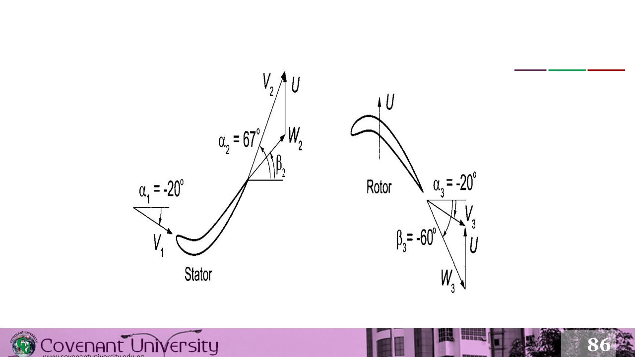
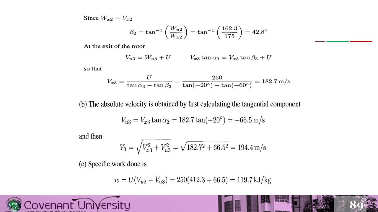
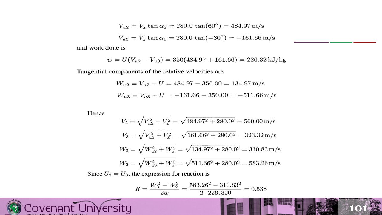
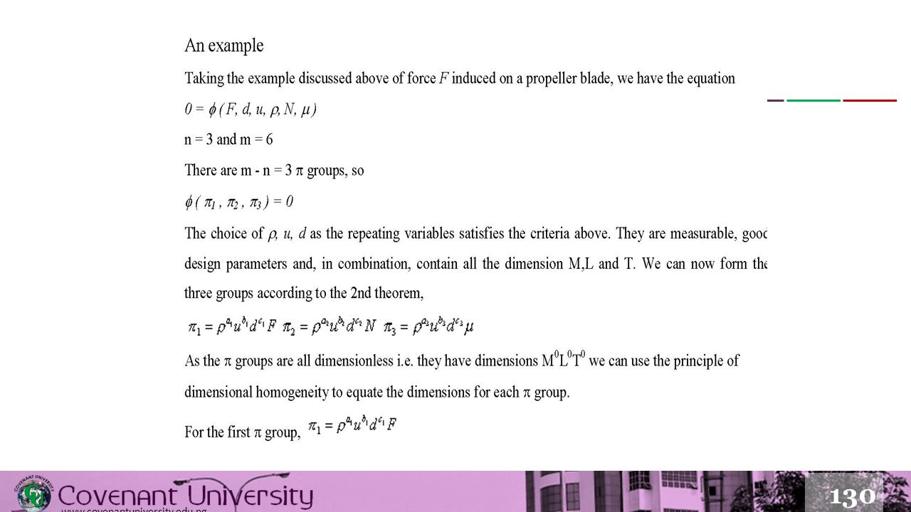
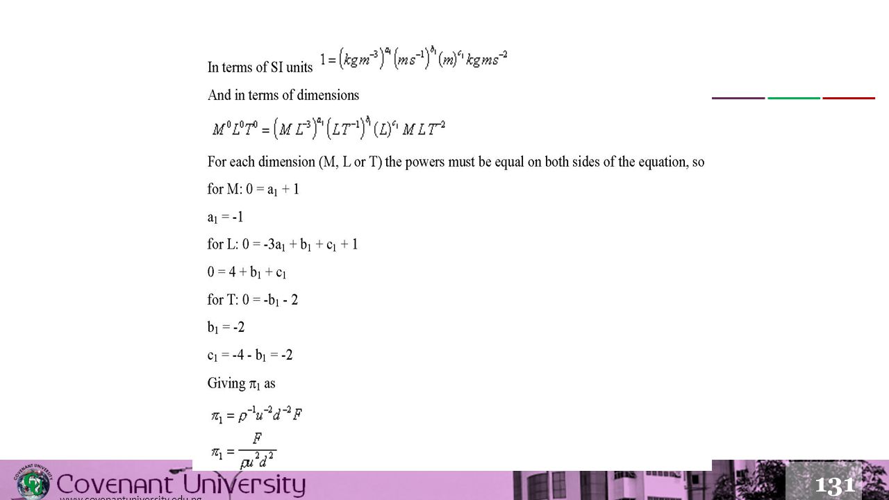


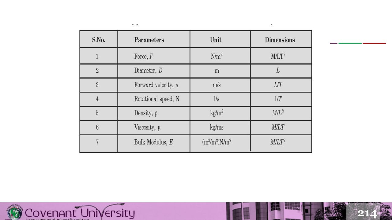
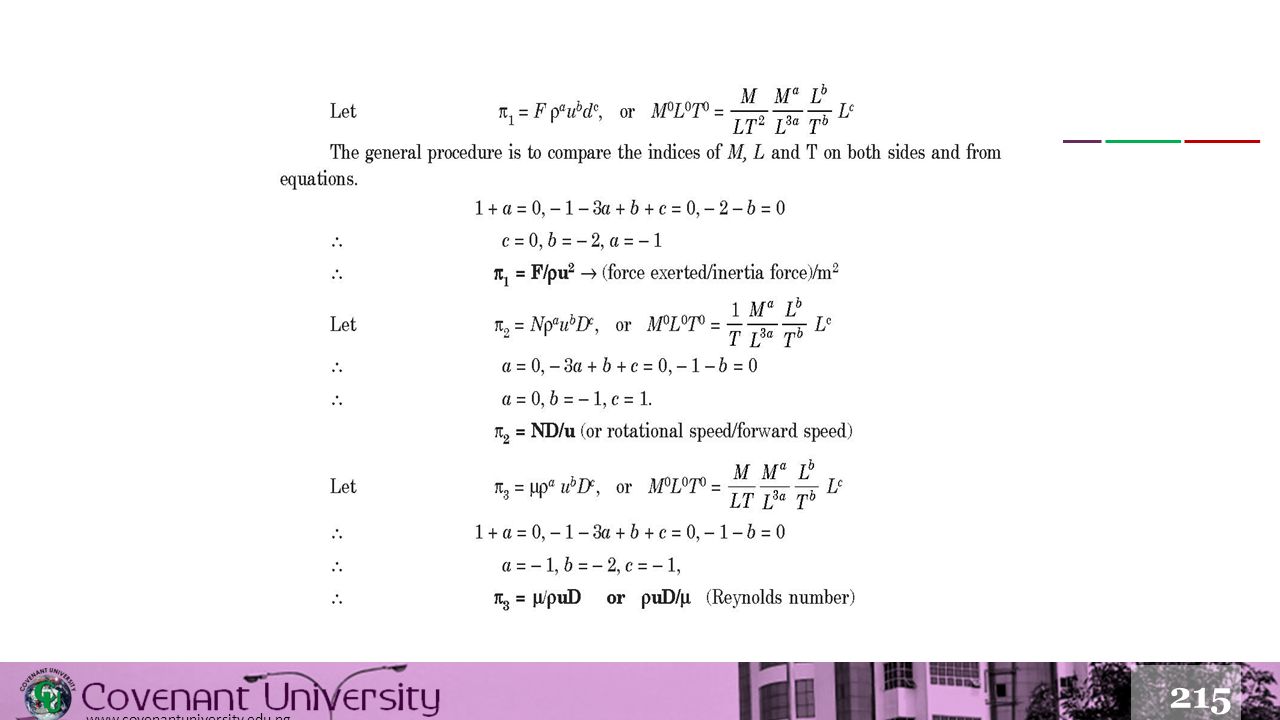

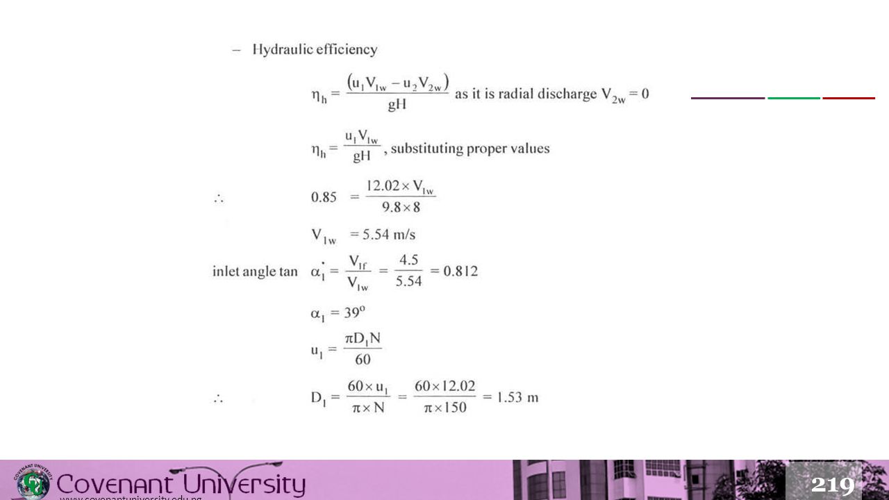
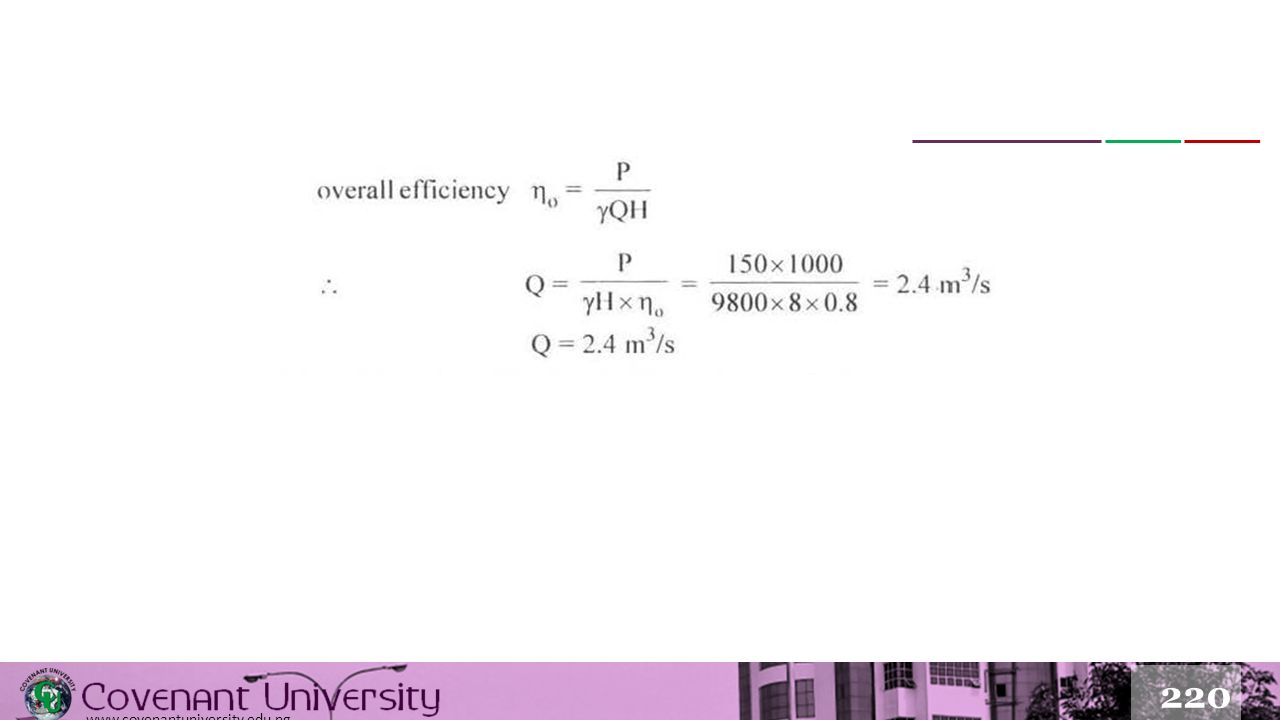


>")


 Tutorial 7.>")


