1. © 2011 Pearson Education, Inc. publishing as Prentice Hall Break-Even Analysis  Technique for evaluating process and equipment alternatives  Objective is to find the point in dollars and units at which cost equals revenue  Requires estimation of fixed costs, variable costs, and revenue

2. © 2011 Pearson Education, Inc. publishing as Prentice Hall Break-Even Analysis  Fixed costs are costs that continue even if no units are produced  Depreciation, taxes, debt, mortgage payments  Variable costs are costs that vary with the volume of units produced  Labor, materials, portion of utilities  Contribution is the difference between selling price and variable cost

3. © 2011 Pearson Education, Inc. publishing as Prentice Hall Break-Even Analysis  Costs and revenue are linear functions  Generally not the case in the real world  We actually know these costs  Very difficult to verify  Time value of money is often ignored Assumptions

4. © 2011 Pearson Education, Inc. publishing as Prentice Hall Profit corridor Loss corridor Break-Even Analysis Total revenue line Total cost line Variable cost Fixed cost Break-even point Total cost = Total revenue – 900 – 800 – 700 – 600 – 500 – 400 – 300 – 200 – 100 – – |||||||||||| 010020030040050060070080090010001100 Cost in dollars Volume (units per period) Figure S7.5

5. © 2011 Pearson Education, Inc. publishing as Prentice Hall Break-Even Analysis BEP x =break-even point in units BEP $ =break-even point in dollars P=price per unit (after all discounts) x=number of units produced TR=total revenue = Px F=fixed costs V=variable cost per unit TC=total costs = F + Vx TR = TC or Px = F + Vx Break-even point occurs when BEP x = F P - V

6. © 2011 Pearson Education, Inc. publishing as Prentice Hall Break-Even Analysis BEP x =break-even point in units BEP $ =break-even point in dollars P=price per unit (after all discounts) x=number of units produced TR=total revenue = Px F=fixed costs V=variable cost per unit TC=total costs = F + Vx BEP $ = BEP x P = P = F (P - V)/P F P - V F 1 - V/P Profit= TR - TC = Px - (F + Vx) = Px - F - Vx = (P - V)x - F

7. © 2011 Pearson Education, Inc. publishing as Prentice Hall Break-Even Example Fixed costs = $10,000 Material = $.75/unit Direct labor = $1.50/unit Selling price = $4.00 per unit BEP $ = F 1 -(V/P) $10,000 1 - [(1.50 +.75)/(4.00)]

8. © 2011 Pearson Education, Inc. publishing as Prentice Hall Break-Even Example Fixed costs = $10,000 Material = $.75/unit Direct labor = $1.50/unit Selling price = $4.00 per unit BEP $ = = F 1 -(V/P) $10,000 1 - [(1.50 +.75)/(4.00)] = $10,000.4375 BEP x = F P - V $10,000 4.00 - (1.50 +.75) = $22,857.14 == 5,714

9. © 2011 Pearson Education, Inc. publishing as Prentice Hall Break-Even Example 50,000 – 40,000 – 30,000 – 20,000 – 10,000 – – |||||| 02,0004,0006,0008,00010,000 Dollars Units Fixed costs Total costs Revenue Break-even point

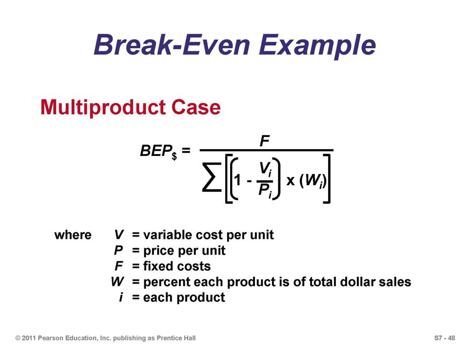
11. © 2011 Pearson Education, Inc. publishing as Prentice Hall Multiproduct Example Annual Forecasted ItemPriceCostSales Units Sandwich$5.00$3.009,000 Drink1.50.509,000 Baked potato2.001.007,000 Fixed costs = $3,000 per month

12. © 2011 Pearson Education, Inc. publishing as Prentice Hall Multiproduct Example Annual Forecasted ItemPriceCostSales Units Sandwich$5.00$3.009,000 Drink1.50.509,000 Baked potato2.001.007,000 Fixed costs = $3,000 per month Sandwich$5.00$3.00.60.40$45,000.621.248 Drinks1.50.50.33.6713,500.186.125 Baked 2.001.00.50.5014,000.193.096 potato $72,5001.000.469 AnnualWeighted SellingVariableForecasted% ofContribution Item (i)Price (P)Cost (V)(V/P)1 - (V/P)Sales $Sales(col 5 x col 7)

13. © 2011 Pearson Education, Inc. publishing as Prentice Hall Multiproduct Example Annual Forecasted ItemPriceCostSales Units Sandwich$5.00$3.009,000 Drink1.50.509,000 Baked potato2.001.007,000 Fixed costs = $3,000 per month Sandwich$5.00$3.00.60.40$45,000.621.248 Drinks1.50.50.33.6713,500.186.125 Baked 2.001.00.50.5014,000.193.096 potato $72,5001.000.469 AnnualWeighted SellingVariableForecasted% ofContribution Item (i)Price (P)Cost (V)(V/P)1 - (V/P)Sales $Sales(col 5 x col 7) BEP $ = F ∑ 1 - x (W i ) ViPiViPi = = $76,759 $3,000 x 12.469 Daily sales = = $246.02 $76,759 312 days.621 x $246.02 $5.00 = 30.6  31 sandwiches per day

14. © 2011 Pearson Education, Inc. publishing as Prentice Hall Expected Monetary Value (EMV) and Capacity Decisions  Determine states of nature  Future demand  Market favorability  Analyzed using decision trees  Hospital supply company  Four alternatives

15. © 2011 Pearson Education, Inc. publishing as Prentice Hall Expected Monetary Value (EMV) and Capacity Decisions -$90,000 Market unfavorable (.6) Market favorable (.4) $100,000 Large plant Market favorable (.4) Market unfavorable (.6) $60,000 -$10,000 Medium plant Market favorable (.4) Market unfavorable (.6) $40,000 -$5,000 Small plant $0 Do nothing

16. © 2011 Pearson Education, Inc. publishing as Prentice Hall Expected Monetary Value (EMV) and Capacity Decisions -$90,000 Market unfavorable (.6) Market favorable (.4) $100,000 Large plant Market favorable (.4) Market unfavorable (.6) $60,000 -$10,000 Medium plant Market favorable (.4) Market unfavorable (.6) $40,000 -$5,000 Small plant $0 Do nothing EMV =(.4)($100,000) + (.6)(-$90,000) Large Plant EMV = -$14,000

17. © 2011 Pearson Education, Inc. publishing as Prentice Hall Expected Monetary Value (EMV) and Capacity Decisions -$90,000 Market unfavorable (.6) Market favorable (.4) $100,000 Large plant Market favorable (.4) Market unfavorable (.6) $60,000 -$10,000 Medium plant Market favorable (.4) Market unfavorable (.6) $40,000 -$5,000 Small plant $0 Do nothing -$14,000 $13,000$18,000

18. © 2011 Pearson Education, Inc. publishing as Prentice Hall Strategy-Driven Investment  Operations may be responsible for return-on-investment (ROI)  Analyzing capacity alternatives should include capital investment, variable cost, cash flows, and net present value

19. © 2011 Pearson Education, Inc. publishing as Prentice Hall Net Present Value (NPV) whereF= future value P= present value i= interest rate N= number of years P = F (1 + i) N F = P(1 + i) N In general: Solving for P:

20. © 2011 Pearson Education, Inc. publishing as Prentice Hall Net Present Value (NPV) whereF= future value P= present value i= interest rate N= number of years P = F (1 + i) N F = P(1 + i) N In general: Solving for P: While this works fine, it is cumbersome for larger values of N

21. © 2011 Pearson Education, Inc. publishing as Prentice Hall NPV Using Factors P = = FX F (1 + i) N whereX=a factor from Table S7.1 defined as = 1/(1 + i) N and F = future value Portion of Table S7.1 Year6%8%10%12%14% 1.943.926.909.893.877 2.890.857.826.797.769 3.840.794.751.712.675 4.792.735.683.636.592 5.747.681.621.567.519

22. © 2011 Pearson Education, Inc. publishing as Prentice Hall Measuring Supply-Chain Performance Table 11.6 Typical Firms Benchmark Firms Lead time (weeks)158 Time spent placing an order42 minutes15 minutes Percentage of late deliveries33%2% Percentage of rejected material1.5%.0001% Number of shortages per year4004

23. © 2011 Pearson Education, Inc. publishing as Prentice Hall Measuring Supply-Chain Performance  Assets committed to inventory Percent invested in inventory = x 100 Total inventory investment Total assets Investment in inventory = $11.4 billion Total assets = $44.4 billion Percent invested in inventory = (11.4/44.4) x 100 = 25.7%

24. © 2011 Pearson Education, Inc. publishing as Prentice Hall Measuring Supply-Chain Performance Table 11.7 Inventory as a % of Total Assets (with exceptional performance) Manufacturing15% (Toyota 5%) Wholesale34% (Coca-Cola 2.9%) Restaurants2.9% (McDonald’s.05%) Retail27% (Home Depot 25.7%)

25. © 2011 Pearson Education, Inc. publishing as Prentice Hall Measuring Supply-Chain Performance  Inventory turnover Inventory turnover = Cost of goods sold Inventory investment

26. © 2011 Pearson Education, Inc. publishing as Prentice Hall Measuring Supply-Chain Performance Table 11.8 Examples of Annual Inventory Turnover Food, Beverage, RetailManufacturing Anheuser Busch15Dell Computer90 Coca-Cola14Johnson Controls22 Home Depot5Toyota (overall)13 McDonald’s112Nissan (assembly)150

27. © 2011 Pearson Education, Inc. publishing as Prentice Hall Measuring Supply-Chain Performance  Inventory turnover Net revenue$32.5 Cost of goods sold$14.2 Inventory: Raw material inventory$.74 Work-in-process inventory$.11 Finished goods inventory$.84 Total inventory investment$1.69

28. © 2011 Pearson Education, Inc. publishing as Prentice Hall Measuring Supply-Chain Performance  Inventory turnover Net revenue$32.5 Cost of goods sold$14.2 Inventory: Raw material inventory$.74 Work-in-process inventory$.11 Finished goods inventory$.84 Total inventory investment$1.69 Inventory turnover = Cost of goods sold Inventory investment = 14.2 / 1.69 = 8.4

29. © 2011 Pearson Education, Inc. publishing as Prentice Hall Measuring Supply-Chain Performance  Inventory turnover Net revenue$32.5 Cost of goods sold$14.2 Inventory: Raw material inventory$.74 Work-in-process inventory$.11 Finished goods inventory$.84 Total inventory investment$1.69 Inventory turnover = Cost of goods sold Inventory investment = 14.2 / 1.69 = 8.4 Weeks of supply = Inventory investment Average weekly cost of goods sold = 1.69 /.273 = 6.19 weeks Average weekly cost of goods sold = $14.2 / 52 = $.273