1. Business Mathematics MTH-367 Lecture 14

2. Last Lecture Summary: Finished Sec. 10.2 and Sec.10.3 Alternative Optimal Solutions No Feasible Solution and Unbounded Solution Scenarios Applications of Linear Programming: – Diet Mix Model – Highway Maintenance (Transportation Model)

3. Chapter 11 The Simplex and Computer Solutions Methods

4. Chapter Objectives Provide an understanding of the simplex method for solving LP problems Illustrate the ways in which special LP phenomena are identified when using the simplex method.

5. Today’s Main Topics We will start Chapter 11 Sec. 11.1: Simplex Preliminaries Overview of the Simplex Method Requirements of Simplex Method Basic feasible solutions Definitions of Feasible Solution; Basic Solution; and Basic Feasible Solution

6. Simplex Preliminaries WHY SIMPLEX METHOD??? ANSWER: Graphical solution methods are applicable to LP problems involving TWO variables The geometry of THREE-variable problems is very complicated, and Beyond Three-variables, there is no geometric frame of reference SO, NEED some NONGRAPHICAL Method...

7. The most popular nongraphical procedure is called The Simplex Method This is an algebraic procedure for solving system of equations where an objective function needs to be optimized. It is an iterative process, which identifies a feasible starting solution.

8. The Simplex Method Cont’d... The procedure then searches to see whether there exists a better solution. “Better” is measured by whether the value of the objective function can be improved. If better solution is signaled, the search resumes The generation of each successive solution requires solving a system of linear equations The search continues until no further improvement is possible in the objective function

9. Requirements of the Simplex Method I.All constraints must be stated as equations. II.The right side of the constraint cannot be negative. III.All variables are restricted to nonnegative values.

10. Most linear programming problems contain constraints which are inequalities. Before we solve by the simplex method, these inequalities must be restated as equations. The transformation from inequalities to equations varies, depending on the nature of the constraints.

11. For each “less than or equal to” constraint, a non-negative variable, called a slack variable, is added to the left side of the constraint. Note that the slack variables become additional variables in the problem and must be treated like any other variables. That means they are also subject to Requirement III; that is, they cannot assume negative values. Transformation procedure for ≤ constraints

12. For each “greater than or equal to” constraint, a non-negative variable E, called a surplus variable, is subtracted from the left side of the constraint. In addition, a non-negative variable A, called an artificial variable, is added to the left of side of the constraint. The artificial variable has no real meaning in the problem; its only function is to provide a convenient starting point (initial guess) for the simplex. Transformation procedure for ≥ constraints

13. .

14. Transformation procedure for = constraints For each “equal to” constraint, an artificial variable, is added to the left of side of the constraint.

15. Example Transform the following constraint set into the standard form required by the simplex method x 1 + x 2 ≤ 100 2x 1 + 3x 2 ≥ 40 x 1 – x 2 = 25 -5x 1 + x 2 ≥ -10 x 1, x 2 ≥ 0

16. Solution Note that each supplemental variable (slack, surplus, artificial) is assigned a subscript which corresponds to the constraint number. Also, the non- negativity restriction (requirement III) applies to all supplemental variables.

17. Requirement II of the simplex method states that the right side of any constraint equation not be negative. If a constraint has a negative right side, the constraint can be multiplied by – 1 to make the right side positive

18. Requirement III of the simplex method states that all variables be restricted to nonnegative values. There are specialize techniques for dealing with variables which can assume negative values; however, we will not examine these methods. The only point which should be repeated is that slack, surplus, and artificial variable are also restricted to being nonnegative.

19. Example An LP problem has 5 decision variables; 10 (≤) constraints; 8 (≥) constraints; and 2 (=) constraints. When this problem is restated to comply with requirement I of the simplex method, how many variables will there be and of what types?

20. Solution There will be 33 variables: 5 decision variables, 10 slack variables associated with the 10 (≤) constraints, 8 surplus variables associated with the 8 (≥) constraints, and 10 artificial variables associated with the (≥) and (=) constraints. 5 + 10 + 8 + 10 = 33

21. Basic Feasible Solutions Let’s state some definitions which are significant to our coming discussions. Assume the standard form of an LP problem which has m structural constraints and a total of n’ decision and supplemental variables. Definition: A feasible solution is any set of values for the n’ variables which satisfies both the structural and non-negativity constraints.

22. Definition: A basic solution is any solution obtained by setting (n’–m) variables equal to 0 and solving the system of equations for the values of the remaining m variables. Definition: The (n’–m) variables which have been assigned values of 0, are called non- basic variables. The rest of the variables are called basic variables. Definition: A basic feasible solution is a basic solution which also satisfies the non-negativity constraints. Thus optimal solution can be found by performing a search of the basic feasible solution.

23. Before we begin our discussions of the simplex method, let’s provide a generalized statement of a LP model. Given the definitions x j = j-th decision variable c j = coefficient on j-th decision variable in the objective function. a ij = coefficient in the i-th constraint for the j-th variable. b i = right-hand-side constant for the i-th constraint THE SIMPLEX METHOD

24. The generalized LP model can be stated as follows: Optimize (maximize or minimize) z = c 1 x 1 + c 2 x 2 +... + c n x n subject to a 11 x 1 + a 12 x 2 +... + a 1n x n (≤, ≥, =) b1(1) a 21 x 1 + a 22 x 2 +... + a 2n x n (≤, ≥, =) b2(2)... a m1 x 1 + a m2 x 2 +... + a mn x n (≤, ≥, =)b m (m) x 1 ≥ 0 x 2 ≥ 0... x n ≥ 0

25. Solution by Enumeration Consider a problem having m (≤) constraints and n variables. Prior to solving by the simplex method, the m constraints would be changed into equations by adding m slack variables. This restatement results in a constraint set consisting of m equations and m + n variables.

26. In Sec. 10.2, we examined the following linear programming problem: Maximizez = 5x 1 + 6x 2 subject to3x 1 + 2x 2 ≤ 120 (1) 4x 1 + 6x 2 ≤ 260 (2) x 1, x 2 ≥ 0 Example

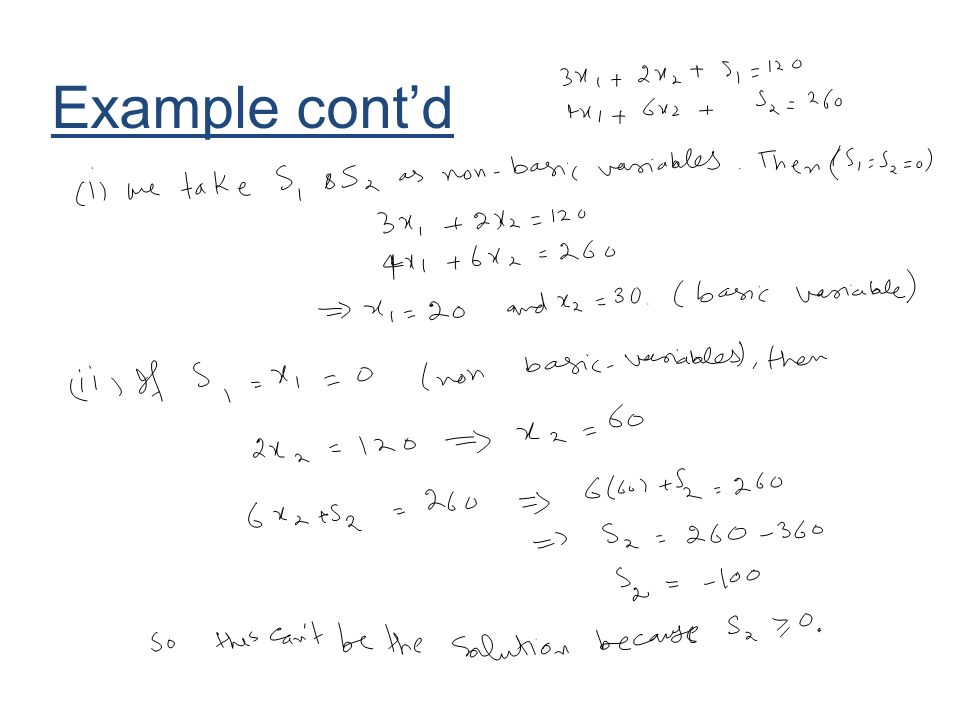
27. Before we solve this problem by the simplex method, the constraint set must be transformed into the equivalent set. 3x 1 + 2x 2 + S 1 = 120 4x 1 + 6x 2 + S 2 = 260 x 1, x 2, S 1, S 2 ≥ 0 The constraint set involves two equations and four variables. Example cont’d

28. Of all the possible solutions to the constraint set, an optimal solution occurs when two of the four variables in this problem are set equal to zero and the system is solved for the other two variables. The question is, which two variables should be set equal to 0 (should be non-basic variables)? Let’s enumerate the different possibilities. Example cont’d

30. Following table summarizes the basic solutions, that is, all the solution possibilities given that two of the four variables are assigned 0 values. SolutionsNon-basic Variables Basic Variables 1S 1, S 2 x 1 = 20, x 2 = 30 *2x 1, S 1 x 2 = 60, S 2 = -100 3x 1, S 2 x 2 = 43.33, S 1 = 33.33 4x 2, S 1 x 1 = 40, S 2 = 100 *5x 2, S 2 x 1 = 65, S 1 = - 75 6x 1, x 2 S 1 = 120, S 2 = 260 Example cont’d

31. Notice that solutions 2 and 5 are not feasible. They each contain a variable which has a negative value, violating the non-negativity restriction. However, solutions 1, 3, 4 and 6 are basic feasible solutions to the linear programming problem and are candidates for the optimal solution. Example cont’d

32. The following figure is the graphical representation of the set of constraints. A (0,6) – Solution 6 (0,43.33) – Solution 3 B (20,30) – Solution 1 C D (40,0) – Solution 4 (65,0) – Solution 5 E F (0,60) – Solution 2 (1) (2) Example cont’d

33. Specifically, solution 1 corresponds to corner point C, solution 3 corresponds to corner point B, solution 4 corresponds to corner point D, and solution 6 corresponds to corner point A. Solution 2 and 5, which are not feasible, correspond to points E and F shown in the figure. Example cont’d

34. Incorporating the Objective Function In solving by the simplex method, the objective function and constraints are combined to form a system of equations. The objective function is one of the equations, and z becomes an additional variable in the system. In rearranging the variables in the objective function so that they are all on the left side of the equation, the problem is represented by the system of equations.

35. z – 5x 1 – 6x 2 – 0S 1 – OS 2 = 0(0) 3x 1 + 2x 2 + S 1 = 120(1) 4x 1 + 6x 2 + S 2 = 260(2) Note: that the objective function is labeled as Eq.(0). The objective is to solve this (3 x 5) system of equations so as to maximize the value of z. Incorporating the Objective Function cont’d

36. Since we are particularly concerned about the value of z and will want to know its value for any solution, z will always be a basic variable. The standard practice, however, is not to refer to z as a basic variable. The terms basic variable and non-basic variable are usually reserved for other variables in the problem. Incorporating the Objective Function cont’d

37. Review We started Chapter 11 Sec. 11.1: Simplex Preliminaries Overview of the Simplex Method Requirements of Simplex Method Basic feasible solutions Definitions of Feasible Solution; Basic Solution; and Basic Feasible Solution Next time, we’ll start Sec 11.2: The Simplex Method