1. Suppose you drive 200 miles, and it takes you 4 hours. Then your average speed is: If you look at your speedometer during this trip, it might read 65 mph. This is your instantaneous speed. 2.1 Rates of Change and Limits

2. A rock falls from a high cliff. The position of the rock is given by: After 2 seconds: average speed: What is the instantaneous speed at 2 seconds? 2.1 Rates of Change and Limits

3. for some very small change in t where h = some very small change in t We can use the TI-84 to evaluate this expression for smaller and smaller values of h. 2.1 Rates of Change and Limits

4. 1 80 0.165.6.0164.16.00164.016.0001 64.0016.0000164.0002 We can see that the velocity approaches 64 ft/sec as h becomes very small. We say that the velocity has a limiting value of 64 as h approaches zero. (Note that h never actually becomes zero.) 2.1 Rates of Change and Limits

5. The limit as h approaches zero: 0 2.1 Rates of Change and Limits

6. Definition: Limit Let c and L be real numbers. The function f has limit L as x approaches c if, for any given positive number ε, there is a positive number δ such that for all x, 2.1 Rates of Change and Limits

7. a L f DNE = Does Not Exist a f L1L1 L2L2 2.1 Rates of Change and Limits

8. Definition: One Sided Limits Left-Hand Limit: The limit of f as x approaches a from the left equals L is denoted Right-Hand Limit: The limit of f as x approaches a from the right equals L is denoted 2.1 Rates of Change and Limits

10. Definition: Limit if and only if and 2.1 Rates of Change and Limits

11. DNE = Does Not Exist Possible Limit Situations a f a f 2.1 Rates of Change and Limits

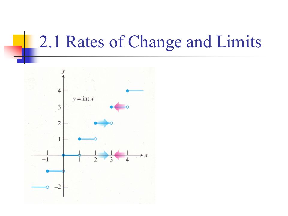
12. 1234 1 2 At x = 1:left hand limit right hand limit value of the function does not exist because the left and right hand limits do not match! 2.1 Rates of Change and Limits

13. At x = 2:left hand limit right hand limit value of the function because the left and right hand limits match. 1234 1 2 2.1 Rates of Change and Limits

14. At x =3 : left hand limit right hand limit value of the function because the left and right hand limits match. 1234 1 2 2.1 Rates of Change and Limits

15. Use your calculator to determine the following: (a) (b) 2.1 Rates of Change and Limits 1 DNE

16. Suppose that c is a constant and the following limits exist 2.1 Rates of Change and Limits

17. Suppose that c is a constant and the following limits exist 2.1 Rates of Change and Limits

18. where n is a positive integer. 2.1 Rates of Change and Limits

19. Evaluate the following limits. Justify each step using the laws of limits. 16 -5/4 2 6 2.1 Rates of Change and Limits

20. 1.If f is a rational function or complex: a.Eliminate common factors. b.Perform long division. c.Simplify the function (if a complex fraction) 2.If radicals exist, rationalize the numerator or denominator. 3.If absolute values exist, use one-sided limits and the following property. 2.1 Rates of Change and Limits

21. 3/2DNE 1/2 DNE 2.1 Rates of Change and Limits

22. Theorem If f(x)  g(x) when x is near a (except possibly at a) and the limits of f and g both exist as x approaches a, then 2.1 Rates of Change and Limits

23. The Squeeze (Sandwich) Theorem If f(x)  g(x)  h(x) when x is near a (except possibly at a) and then 2.1 Rates of Change and Limits

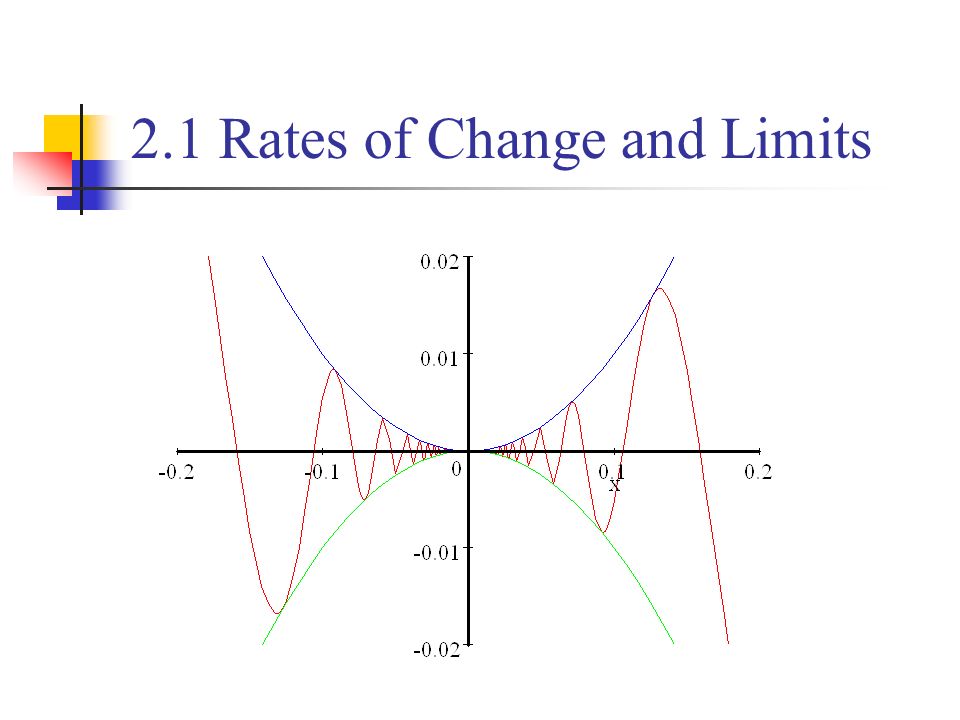
24. Show that: The maximum value of sine is 1, soThe minimum value of sine is -1, soSo: 2.1 Rates of Change and Limits

25. By the sandwich theorem: 2.1 Rates of Change and Limits

27. Therefore, 2.1 Rates of Change and Limits

28. simplify and divide by sin θ 2.1 Rates of Change and Limits

29. P(cos , sin  ) Q(1,0) 

30. The notation means that the values of f(x) can be made arbitrarily large (as large as we please) by taking x sufficiently close to a (on either side) but not equal to a. 2.2 Limits Involving Infinity

31. a f Vertical Asymptote 2.2 Limits Involving Infinity

32. Vertical Asymptote The line x = a is called a vertical asymptote of the curve y = f(x) if at least one of the following statements is true: 2.2 Limits Involving Infinity

33. f(x) = ln x has a vertical asymptote at x = 0 since f(x) = tan x has a vertical asymptote at x =  /2 since 2.2 Limits Involving Infinity

34. -∞-∞ x = 3 x = 1 Determine the equations of the vertical asymptotes of Find the limit

35. Let f be a function defined on some interval (a, ∞). Then means that the value of f(x) can be made as close to L as we like by taking x sufficiently large. 2.2 Limits Involving Infinity

36. Horizontal Asymptote L f 2.2 Limits Involving Infinity

37. Definition End Behavior Model Suppose that f is a rational function as follows:

38. Horizontal Asymptote The line y = L is called a horizontal asymptote of the curve y = f(x) if either or 2.2 Limits Involving Infinity

39. f(x) = e x has a horizontal asymptote at y = 0 since 2.2 Limits Involving Infinity

40. If n is a positive integer, then 2.2 Limits Involving Infinity

41. Find the limit 2.2 Limits Involving Infinity -1/3 2/3 1/3

42. Find the limit 2.2 Limits Involving Infinity Use squeeze theorem

43. 2.2 Limits Involving Infinity

44. A function is continuous at a point if the limit is the same as the value of the function. This function has discontinuities at x = 1 and x = 2. It is continuous at x = 0 and x =4, because the one-sided limits match the value of the function 1234 1 2 2.3 Continuity

45. Definition: Continuity A function is continuous at a number a if That is, 1.f(a) is defined 2. exists 3. 2.3 Continuity

46. Definition: One Sided Continuity A function f is continuous from the right at a number a if and f is continuous from the left at a if 2.3 Continuity

47. 1. Removable discontinuity 2.3 Continuity

48. 2. Infinite discontinuity 2.3 Continuity

49. 3. Jump discontinuity 2.3 Continuity

50. 4. Oscillating discontinuity 2.3 Continuity

51. Definition: Continuity On An Interval A function f is continuous on an interval if it is continuous at every number in the interval. (If f is defined on one side of an endpoint of the interval, we understand continuous at the endpoints to mean continuous from the right or continuous from the left). 2.3 Continuity

52. Theorem 1. f + g 2. f – g 3. cf 4. fg 5. f / g if g(a)  0 6. f(g(x)) If f and g are continuous at a and c is a constant, then the following functions are also continuous at a: 2.3 Continuity

53. Theorem (a)Any polynomial is continuous everywhere; that is, it is continuous on  = (-∞, ∞). (b)Any rational function is continuous whenever it is defined; that is, it is continuous on its domain. 2.3 Continuity

54. Any of the following types of functions are continuous at every number in their domain: Polynomials; Rational Functions, Root Functions; Trigonometric Functions; Inverse Trigonometric Functions; Exponential Functions; and Logarithmic Functions. 2.3 Continuity

55. If f is continuous at b and, then. In other words, 2.3 Continuity

56. If g is continuous at a and f is continuous at g(a), then the composite function f(g(x)) is continuous at a. 2.3 Continuity

57. The Intermediate Value Theorem Suppose that f is continuous on the closed interval [a, b] and let N be any number between f(a) and f(b). Then there exists a number c in (a, b) such that f(c) = N. a f b f(a)f(a) f(b)f(b) c f(c)=N 2.3 Continuity

58. Use the Intermediate Value Theorem to show that there is a root of the given equation in the specified interval. 2.3 Continuity

59. Graph Continuous at x=0?

60. Graph Continuous at x = 0? 00 yes undefined0no undefinedDNEno undefined 1 no 00 yes undefined 1no undefined DNE no 0DNE no undefined 0 no

61. Definition: Limit Let c and L be real numbers. The function f has limit L as x approaches c if, for any given positive number ε, there is a positive number δ such that for all x, 2.3 Continuity

62. Solution Set c = 1 and f(x) = 5x - 3 and L = 2. For any given  > 0, there exists a  > 0 such that 0 < |x - 1| <  whenever |f(x) - 2| <  2.3 Continuity

63. |(5x - 3) - 2| <  |5x - 5| <  5|x - 1| <  |x - 1| <  /5 So if  =  /5 1-  1 1+  2+  2-  2 2.3 Continuity

64. Solution Set c = 2 and f(x) = 3x - 1 and L = 5. For any given  > 0, there exists a  > 0 such that 0 < |x - 2| <  whenever |f(x) - 5| <  2.3 Continuity

65. |(3x - 1) - 5| <  |3x - 6| <  3|x - 2| <  |x - 2| <  /3 So if  =  /3 2-  2 2+  5+  5-  5 2.3 Continuity

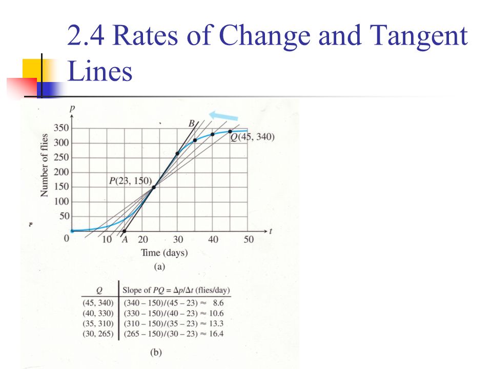
66. Definition Average Rate of Change The average rate of change of a quantity over a period of time is the amount of change divided by the time it takes. 2.4 Rates of Change and Tangent Lines

67. Find the average rate of change of f(x) = x 2 - 2x over the interval [1,3] and the equation of the secant line. f(1) = -1 f(3) = 3 (3,3) (1,-1) y = mx + b3 = 2*3 + b b = -3y = 2x - 3 2.4 Rates of Change and Tangent Lines

69. Slope of a Curve Definition Slope of a Curve at a Point The slope of the curve y = f(x) at the point P(a, f(a)) is provided the limit exists or The tangent line to the curve at P is the line through P with this slope. 2.4 Rates of Change and Tangent Lines

70. Find the slope of the parabola y = x 2 at the point (2,4) 2.4 Rates of Change and Tangent Lines Demonstration

71. 2.4 Rates of Change and Tangent Lines

72. Normal to a curve The normal line to a curve at a point is the line perpendicular to the tangent at that point. 2.4 Rates of Change and Tangent Lines

73. Find an equation of the normal line to the curve y = 9 – x 2 at x = 2 2.4 Rates of Change and Tangent Lines

74. At x = 2, the slope of the tangent line is -2(2) = -4, so the slope of the normal line is ¼. y = mx + b 5= (1/4) (2) + b 5= 1/2 + b b = 9/2 y= (1/4) x + 9/2 2.4 Rates of Change and Tangent Lines