1. Artificial Intelligence Lecture 5: Search Methods III Faculty of Mathematical Sciences 4 th 5 th IT Elmuntasir Abdallah Hag Eltom

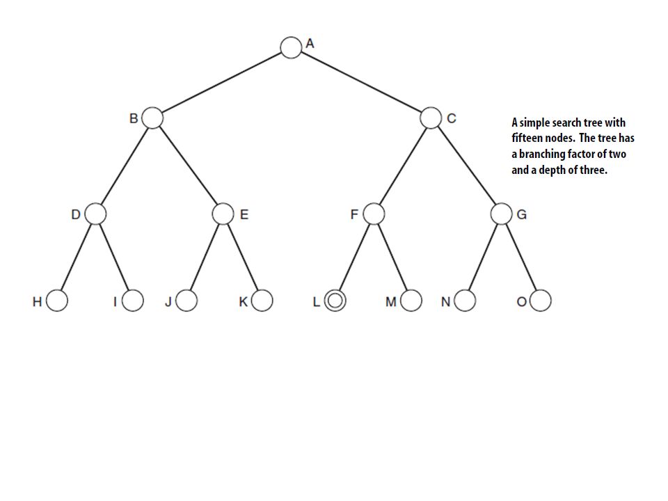
2. Lecture Objectives [Part II: Chapter 4] Introduce a number of search methods, including depth-first search and breadth-first search. Metrics are presented that enable analysis of search methods and provide a way to determine which search methods are most suitable for particular problems. Introduce the idea of heuristics for search and presents a number of methods, such as best- first search, that use heuristics to improve the performance of search methods.

3. Introduction to search methods We have introduced search trees and other methods and representations that are used for solving problems using Artificial Intelligence techniques such as search. We will discuss how effective they are in different situations. Depth-first search and breadth-first search are the best-known and widest-used search methods, we will examine why this is and how they are implemented. We also look at a number of properties of search methods, including optimality and completeness, that can be used to determine how useful a search method will be for solving a particular problem.

4. Introduction to search methods Search methods have impact on almost every aspect of Artificial Intelligence. Because of the serial nature in which computers tend to operate, search is a necessity to determine solutions to an enormous range of problems. We will start by discussing blind search methods and moves on to examine search methods that are more informed—these search methods use heuristics to examine a search space more efficiently.

5. Problem Solving as Search A problem can be considered to consist of a goal and a set of actions that can be taken to lead to the goal. At any given time, we consider the state of the search space to represent where we have reached as a result of the actions we have applied so far.

6. Problem Solving as Search Consider the problem of looking for a contact lens on a football field. The initial state is how we start out, which is to say we know that the lens is somewhere on the field, but we don’t know where. If we use the representation where we examine the field in units of one square foot, then our first action might be to examine the square in the top-left corner of the field. If we do not find the lens there, we could consider the state now to be that we have examined the top-left square and have not found the lens. After a number of actions, the state might be that we have examined 500 squares, and we have now just found the lens in the last square we examined. This is a goal state because it satisfies the goal that we had of finding a contact lens.

7. Problem Solving as Search Search is a method that can be used by computers to examine a problem space (like this) in order to find a goal. Often, we want to find the goal as quickly as possible or without using too many resources. A problem space can also be considered to be a search space because in order to solve the problem, we will search the space for a goal state. We will continue to use the term search space to describe this concept.

8. Data-Driven or Goal-Driven Search There are two main approaches to searching a search tree, corresponding to top-down and bottom-up approaches. Data-driven search starts from an initial state (root node) and uses actions that are allowed to move forward until a goal (goal node) is reached. This approach is also known as forward chaining. Alternatively, search can start at the goal and work back toward a start state, by seeing what moves could have led to the goal state. This is goal-driven search, also known as backward chaining.

9. Data-Driven or Goal-Driven Search Goal-driven search and data-driven search will end up producing the same results. Depending on the nature of the problem being solved, in some cases one can run more efficiently than the other—in particular, in some situations one method will involve examining more states than the other.

10. Example Situations for Goal- Driven Search Goal-driven search is particularly useful in situations in which the goal can be clearly specified (for example, a theorem that is to be proved or finding an exit from a maze). It is also clearly the best choice in situations such as medical diagnosis where the goal (the condition to be diagnosed) is known, but the rest of the data (in this case, the causes of the condition) need to be found.

11. Example Situations for Data- Driven Search Data-driven search is most useful when the initial data are provided, and it is not clear what the goal is. For example, a system that analyzes astronomical data and thus makes deductions about the nature of stars and planets would receive a great deal of data, but it would not necessarily be given any direct goals. Rather, it would be expected to analyze the data and determine conclusions of its own. This kind of system has a huge number of possible goals that it might locate. In this case, data-driven search is most appropriate.

12. Example Situations for Data- Driven Search It is interesting to consider a maze that has been designed to be traversed from a start point in order to reach a particular end point. It is nearly always far easier to start from the end point and work back toward the start point. This is because a number of dead end paths have been set up from the start (data) point, and only one path has been set up to the end (goal) point. As a result, working back from the goal to the start has only one possible path.

13. Generate and Test The simplest approach to search is called Generate and Test. This simply involves generating each node in the search space and testing it to see if it is a goal node. If it is, the search has succeeded and need not carry on. Otherwise, the procedure moves on to the next node.

14. Generate and Test This is the simplest form of brute-force search (also called exhaustive search), so called because it assumes no additional knowledge other than how to traverse the search tree and how to identify leaf nodes and goal nodes. Generate and test [Brute-force] will ultimately examine every node in the tree until it finds a goal.

15. Generate and Test [Generator] To successfully operate, Generate and Test needs to have a suitable Generator, which should satisfy three properties: 1. It must be complete: In other words, it must generate every possible solution; otherwise it might miss a suitable solution. 2. It must be nonredundant: This means that it should not generate the same solution twice. 3. It must be well informed: This means that it should only propose suitable solutions and should not examine possible solutions that do not match the search space.

16. Generate and Test Problems The Generate and Test method can be successfully applied to a number of problems and indeed is the manner in which people often solve problems where there is no additional information about how to reach a solution.

17. Generate and Test Example If you know that a friend lives on a particular road, but you do not know which house, a Generate and Test approach might be necessary. This would involve ringing the doorbell of each house in turn until you found your friend. Similarly, Generate and Test can be used to find solutions to combinatorial problems such as the eight queens problem. Generate and Test is also sometimes referred to as a blind search technique because of the way in which the search tree is searched without using any information about the search space.

18. Depth-First Search Depth-first search is so called because it follows each path to its greatest depth before moving on to the next path. The principle behind the depth-first approach is illustrated in next slide.

19. Depth-First Search Assuming that we start from the left side and work toward the right, depth-first search involves working all the way down the left-most path in the tree until a leaf node is reached. If this is a goal state, the search is complete, and success is reported.

20. Depth-First Search If the leaf node does not represent a goal state, search backtracks up to the next highest node that has an unexplored path. In previous slide, after examining node G and discovering that it is not a goal node, search will backtrack to node D and explore its other children. In this case, it only has one other child, which is H. Once this node has been examined, search backtracks to the next unexpanded node, which is A, because B has no unexplored children.

21. Depth-First Search This process continues until either all the nodes have been examined, in which case the search has failed, or until a goal state has been reached, in which case the search has succeeded. In (previous depth-first search diagram), search stops at node J, which is the goal node. As a result, nodes F, K, and L are never examined.

22. Chronological Backtracking Depth-first search uses a method called chronological backtracking to move back up the search tree once a dead end has been found. Chronological backtracking is so called because it undoes choices in reverse order of the time the decisions were originally made. We will see later in this chapter that nonchronological backtracking, where choices are undone in a more structured order, can be helpful in solving certain problems. Depth-first search is an example of brute-force search, or exhaustive search.

23. Depth-First Search Depth-first search is often used by computers for search problems such as locating files on a disk, or by search engines for spidering the Internet. As anyone who has used the find operation on their computer will know, depth-first search can run into problems. In particular, if a branch of the search tree is extremely large, or even infinite, then the search algorithm will spend an inordinate amount of time examining that branch, which might never lead to a goal state.

24. Breadth-First Search An alternative to depth-first search is breadth-first search. As its name suggests, this approach involves traversing a tree by breadth rather than by depth. As can be seen from next slide, the breadth-first algorithm starts by examining all nodes one level (sometimes called one ply) down from the root node.

25. Breadth-First Search If a goal state is reached here, success is reported. Otherwise, search continues by expanding paths from all the nodes in the current level down to the next level. In this way, search continues examining nodes in a particular level, reporting success when a goal node is found, and reporting failure if all nodes have been examined and no goal node has been found.

26. Breadth-First Search Breadth-first search is a far better method to use in situations where the tree may have very deep paths, and particularly where the goal node is in a shallower part of the tree. It does not perform so well where the branching factor of the tree is extremely high, such as when examining game trees for games like Go or Chess. Breadth-first search is a poor idea in trees where all paths lead to a goal node with similar length paths. In situations such as this, depth-first search would perform far better because it would identify a goal node when it reached the bottom of the first path it examined.

27. Comparison between Depth-First and Breadth-First Search Depth-first search is usually simpler to implement than breadth-first search. –It usually requires less memory usage because it only needs to store information about the path it is currently exploring, whereas breadth-first search needs to store information about all paths that reach the current depth. –This is one of the main reasons that depth-first search is used so widely to solve everyday computer problems.

28. Infinite path The problem of infinite paths can be avoided in depth- first search by applying a depth threshold. This means that paths will be considered to have terminated when they reach a specified depth. This has the disadvantage that some goal states (or, in some cases, the only goal state) might be missed but ensures that all branches of the search tree will be explored in reasonable time. This technique is often used when examining game trees.

29. Properties of Search Methods Different search methods perform in different ways. There are several important properties that search methods should have in order to be most useful. ■ Complexity ■ Completeness ■ Optimality ■ Admissibility ■ Irrevocability

30. Complexity In discussing a search method, it is useful to describe how efficient that method is, over time and space. The time complexity of a method is related to the length of time that the method would take to find a goal state. The space complexity is related to the amount of memory that the method needs to use. It is normal to use Big-O notation to describe the complexity of a method. For example, breadth- first search has a time complexity of O(b d ), where b is the branching factor of the tree, and d is the depth of the goal node in the tree

31. Complexity Depth-first search is very efficient in space because it only needs to store information about the path it is currently examining, but it is not efficient in time because it can end up examining very deep branches of the tree.

32. Complexity Clearly, complexity is an important property to understand about a search method. A search method that is very inefficient may perform reasonably well for a small test problem, but when faced with a large real-world problem, it might take an unacceptably long period of time. As we will see, there can be a great deal of difference between the performance of two search methods, and selecting the one that performs the most efficiently in a particular situation can be very important.

33. Complexity This complexity must often be weighed against the adequacy of the solution generated by the method. A very fast search method might not always find the best solution, whereas, for example, a search method that examines every possible solution will guarantee to find the best solution, but it will be very inefficient

34. Completeness A search method is described as being complete if it is guaranteed to find a goal state if one exists. Breadth-first search is complete, but depth-first search is not because it may explore a path of infinite length and never find a goal node that exists on another path.

35. Completeness Completeness is usually a desirable property because running a search method that never finds a solution is not often helpful. On the other hand, it can be the case (as when searching a game tree, when playing a game, for example) that searching the entire search tree is not necessary, or simply not possible, in which case a method that searches enough of the tree might be good enough. A method that is not complete has the disadvantage that it cannot necessarily be believed if it reports that no solution exists.

36. Optimality A search method is optimal if it is guaranteed to find the best solution that exists. In other words, it will find the path to a goal state that involves taking the least number of steps. This does not mean that the search method itself is efficient—it might take a great deal of time for an optimal search method to identify the optimal solution—but once it has found the solution, it is guaranteed to be the best one.

37. Optimality This is fine if the process of searching for a solution is less time consuming than actually implementing the solution. On the other hand, in some cases implementing the solution once it has been found is very simple, in which case it would be more beneficial to run a faster search method, and not worry about whether it found the optimal solution or not.

38. Optimality Breadth-first search is an optimal search method, but depth-first search is not. Depth-first search returns the first solution it happens to find, which may be the worst solution that exists. Because breadth-first search examines all nodes at a given depth before moving on to the next depth, if it finds a solution, there cannot be another solution before it in the search tree. In some cases, the word optimal is used to describe an algorithm that finds a solution in the quickest possible time, in which case the concept of admissibility is used in place of optimality. An algorithm is then defined as admissible if it is guaranteed to find the best solution.

39. Irrevocability Methods that use backtracking are described as tentative. Methods that do not use backtracking, and which therefore examine just one path, are described as irrevocable. Depth-first search is an example of tentative search. Irrevocable search methods will often find suboptimal solutions to problems because they tend to be fooled by local optima-solutions that look good locally but are less favorable when compared with other solutions elsewhere in the search space.

40. Why Humans Use Depth-First Search? Depth-first search is somewhat easier. It is also somewhat easier for humans to understand because it much more closely relates to the natural way in which humans search for things, as we see in the following two examples.

41. Example 1: Traversing a Maze When traversing a maze, most people will wander randomly, hoping they will eventually find the exit. This approach will usually be successful eventually but is not the most rational and often leads to what we call “going round in circles.” This problem relates to search spaces that contain loops, and it can be avoided by converting the search space into a search tree.

42. Example 1: Traversing a Maze

43. An alternative method is: To start with your hand on the left side of the maze (or the right side, if you prefer). Follow the maze around, always keeping your left hand on the left edge of the maze wall. In this way, you are guaranteed to find the exit. This is because this technique corresponds exactly to depth-first search.

44. Example 1: Traversing a Maze Certain special points in the maze have been labeled: ■ A is the entrance to the maze. ■ M is the exit from the maze. ■ C, E, F, G, H, J, L, and N are dead ends. ■ B, D, I, and K are points in the maze where a choice can be made as to which direction to go next.

45. Example 1: Traversing a Maze In following the maze by running one’s hand along the left edge, the following path would be taken: A, B, E, F, C, D, G, H, I, J, K, L,M

46. Example 1: Traversing a Maze You should be able to see that following the search tree using depth-first search takes the same path. This is only the case because the nodes of the search tree have been ordered correctly. The ordering has been chosen so that each node has its left-most child first and its right-most child last. Using a different ordering would cause depth- first search to follow a different path through the maze.

47. Example 2: Searching for a Gift When looking for a present for a relative in a number of shops, each of which has several floors, and where each floor has several departments, depth-first search might be a natural, if rather simplistic, approach This would involve visiting each floor in the first building before moving on to the next building.

48. Example 2: Searching for a Gift A breadth-first approach would mean examining the first department in each shop, and then going back to examine the second department in each shop, and so on. This way does not make sense due to the spatial relationship between the departments, floors, and shops. For a computer, either approach would work equally well as long as a representation was used where moving from one building to another did not take any computation time.

49. Example 2: Searching for a Gift In both of the examples above, it can be seen that using breadth-first search, although a perfectly reasonable approach for a computer system, would be rather strange for a human. This is probably because with depth-first search, the approach is to explore each path fully before moving onto another path, whereas with breadth-first search, the approach involves revisiting and extending particular paths many times. Despite this, implementations in software of both algorithms are nearly identical, at least when expressed in pseudocode.

51. Implementing Depth-First and Breadth-First Search The variable state represents the current state at any given point in the algorithm, and queue is a data structure that stores a number of states, in a form that allows insertion and removal from either end. In this algorithm, we always insert at the front and remove from the front, which as we will see later on means that depth-first search can be easily implemented using a stack. In this implementation, we have used the function successors (state),which simply returns all successors of a given state.

52. Function depth () { queue = []; // initialize an empty queue state = root_node; // initialize the start state while (true) { if is_goal (state) then return SUCCESS else add_to_front_of_queue (successors (state)); if queue == [] then report FAILURE; state = queue [0]; // state = first item in queue remove_first_item_from (queue); }

53. In fact, depth-first search can be readily implemented on most computer systems using a stack, which is simply a “last in first out” queue (sometimes called a LIFO). In this way, a recursive version of the algorithm given above can be used, as follows. Because this function is recursive, it needs to be called with an argument: recursive_depth (root_node); The function is defined as follows: Implementing Depth-First and Breadth-First Search

54. Function recursive_depth (state) { if is_goal (state) then return SUCCESS else { remove_from_stack (state); add_to_stack (successors (state)) } while (stack != []) { if recursive_depth (stack [0]) == SUCCESS then return SUCCESS; remove_first_item_from (stack); } return FAILURE; }

56. Topics to read Implementation of breadth-first. Web Spidering example.

57. Depth-First Iterative Deepening Depth-First Iterative Deepening, or DFID (also called Iterative Deepening Search or IDS), is an exhaustive search technique that combines depth-first with breadth- first search. The DFID algorithm involves repeatedly carrying out depth-first searches on the tree, starting with a depth- first search limited to a depth of one, then a depth-first search of depth two, and so on, until a goal node is found. This is an algorithm that appears to be somewhat wasteful in terms of the number of steps that are required to find a solution. However, it has the advantage of combining the efficiency of memory use of depth-first search with the advantage that branches of the search tree that are infinite or extremely large will not sidetrack the search.

58. Using Heuristics for Search Depth-first and breadth-first search were described as brute-force search methods because they do not employ any special knowledge of the search trees they are examining but simply examine every node in order until they happen upon the goal. This can be likened to the human being who is traversing a maze by running a hand along the left side of the maze wall.

59. Using Heuristics for Search Take the example of looking for a suitable gift. Very few people would simply walk into each shop as they came across it, looking in each department in turn until they happened upon a present. Most people would go straight to the shop that they considered to be most likely to have a suitable gift. If no gift was found in that shop, they would then proceed to the shop they considered to be the next most likely to have a suitable gift.

60. Using Heuristics for Search This kind of information is called a heuristic, and humans use them all the time to solve all kinds of problems. Computers can also use heuristics, and in many problems heuristics can reduce an otherwise impossible problem to a relatively simple one.

61. Using Heuristics for Search A heuristic evaluation function is a function that when applied to a node gives a value that represents a good estimate of the distance of the node from the goal. For two nodes m and n, and a heuristic function f, if f(m) < f(n), then it should be the case that m is more likely to be on an optimal path to the goal node than n. In other words, the lower the heuristic value of a node, the more likely it is that it is on an optimal path to a goal and the more sensible it is for a search method to examine that node.

62. Using Heuristics for Search The following sections provide details of a number of search methods that use heuristics and are thus thought of as heuristic search methods, or heuristically informed search methods. Typically, the heuristic used in search is one that provides an estimate of the distance from any given node to a goal node. This estimate may or may not be accurate, but it should at least provide better results than pure guesswork.

63. Informed and Uninformed Methods A search method or heuristic is informed if it uses additional information about nodes that have not yet been explored to decide which nodes to examine next. If a method is not informed, it is uninformed, or blind. In other words, search methods that use heuristics are informed, and those that do not are blind. Best-first search is an example of informed search, whereas breadth-first and depth-first search are uninformed or blind.

64. Informed and Uninformed Methods A heuristic h is said to be more informed than another heuristic, j, if: –h(node) ≥ j(node) for all nodes in the search space. –(In fact, in order for h to be more informed than j, there must be some node where h(node) > j(node). Otherwise they are as informed as each other.) The more informed a search method is, the more efficiently it will search.

65. Choosing a Good Heuristic In choosing heuristics, we usually consider that a heuristic that reduces the number of nodes that need to be examined in the search tree is a good heuristic. It is also important to consider the efficiency of running the heuristic itself. In other words, if it takes an hour to compute a heuristic value for a given state, the fact that doing so saves a few minutes of total search time is irrelevant. we will assume that heuristic functions we choose are extremely simple to calculate and so do not impact on the overall efficiency of the search algorithm.