2. HST.582J/6.555J/16.456J Gari D. Clifford Associate Director, Centre for Doctoral Training, IBME, University of Oxford gari@alum.mit.edu http://alum.mit.edu/www/gari © G. D. Clifford 2005-2011 Blind Source Separation: PCA & ICA

3. What is BSS? Assume an observation (signal) is a linear mix of >1 unknown independent source signals The mixing (not the signals) is stationary We have as many observations as unknown sources To find sources in observations - need to define a suitable measure of independence … For example - the cocktail party problem (sources are speakers and background noise):

4. The cocktail party problem - find Z A z1z1 z2z2 zNzN XTXT ZTZT X T =AZ T x1x1 x2x2 xNxN

5. Formal statement of problem N independent sources … Z mn ( M xN ) linear square mixing … A nn ( N xN ) (#sources=#sensors) produces a set of observations … X mn ( M xN ) ….. X T = AZ T

6. Formal statement of solution ‘demix’ observations … X T ( N xM ) into Y T = WX T Y T ( N xM )  Z T W ( N xN )  A -1 How do we recover the independent sources? (We are trying to estimate W  A -1 ) …. We require a measure of independence!

7. ‘Signal’ source ‘Noise’ sources Observed mixtures ZTZT X T =AZ T Y T =WX T

8. X T = A Z T Y T = W X T TT TT

9. The Fourier Transform (Independence between components is assumed)

10. Recap: Non-causal Wiener filtering x[n] - observation y[n] - ideal signal d[n] - noise component Ideal Signal S y (f ) Noise Power S d (f ) Observation S x (f ) Filtered signal: S filt (f ) = S x (f ).H(f ) f

11. BSS is a transform? Like Fourier, we decompose into components by transforming the observations into another vector space which maximises the separation between interesting (signal) and unwanted (noise). Unlike Fourier, separation is not based on frequency- It’s based on independence Sources can have the same frequency content No assumptions about the signals (other than they are independent and linearly mixed) So you can filter/separate in-band noise/signals with BSS

12. Principal Component Analysis Second order decorrelation = independence Find a set of orthogonal axes in the data (independence metric = variance) Project data onto these axes to decorrelate Independence is forced onto the data through the orthogonality of axes Conventional noise / signal separation technique

13. Singular Value Decomposition Decompose observation X=AZ into…. X=USV T S is a diagonal matrix of singular values with elements arranged in descending order of magnitude (the singular spectrum) The columns of V are the eigenvectors of C=X T X (the orthogonal subspace … dot(v i,v j )=0 ) … they ‘demix’ or rotate the data U is the matrix of projections of X onto the eigenvectors of C … the ‘source’ estimates

14. Singular Value Decomposition Decompose observation X=AZ into…. X=USV T

15. Eigenspectrum of decomposition S = singular matrix … zeros except on the leading diagonal S ij (i=j) are the eigenvalues ½ Placed in order of descending magnitude Correspond to the magnitude of projected data along each eigenvector Eigenvectors are the axes of maximal variation in the data Variance = power (analogous to Fourier components in power spectra) [stem(diag(S).^2)] Eigenspectrum= Plot of eigenvalues

16. SVD: Method for PCA

17. SVD noise/signal separation To perform SVD filtering of a signal, use a truncated SVD decomposition (using the first p eigenvectors) Y=US p V T [Reduce the dimensionality of the data by discarding noise projections S noise =0 Then reconstruct the data with just the signal subspace] Most of the signal is contained in the first few principal components. Discarding these and projecting back into the original observation space effects a noise-filtering or a noise/signal separation

18. Real data Add noise

19. Real data X X p =US p V T S2S2 X p … p=2 n X p … p=4

20. Two dimensional example

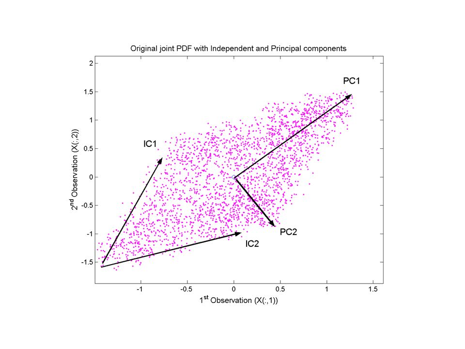
23. Independent Component Analysis As in PCA, we are looking for N different vectors onto which we can project our observations to give a set of N maximally independent signals (sources) output data (discovered sources) dimensionality = dimensionality of observations Instead of using variance as our independence measure (i.e. decorrelating) as we do in PCA, we use a measure of how statistically independent the sources are.

24. ICA: The basic idea... Assume underlying source signals (Z ) are independent. Assume a linear mixing matrix (A )… X T =AZ T in order to find Y (  Z ), find W, (  A -1 )... Y T =WX T How? Initialise W & iteratively update W to minimise or maximise a cost function that measures the (statistical) independence between the columns of the Y T.

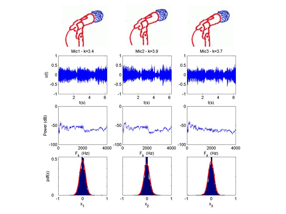
25. Non-Gaussianity  statistical independence? From the Central Limit Theorem, - add enough independent signals together, Gaussian PDF Sources, Z P(Z) ( subGaussian ) Mixtures (X T =AZ T ) P(X) ( Gaussian )

26. Recap: Moments of a distribution

27. Higher order moments (3 rd -skewness) xx

28. Higher order moments (4 th -kurtosis) xx SuperGaussianSubGaussian Gaussians are mesokurtic with κ =3

29. Non-Gaussianity  statistical independence? Central Limit Theorem: add enough independent signals together, Gaussian PDF  make data components non-Gaussian to find independent sources Sources, Z P(Z) (  <3 (1.8) ) Mixtures (X T =AZ T ) P(X) (  =3.4) (  =3)

30. Recall – trying to estimate W Assume underlying source signals (Z ) are independent. Assume a linear mixing matrix (A )… X T =AZ T in order to find Y (  Z ), find W, (  A -1 )... Y T =WX T Initialise W & iteratively update W with gradient descent to maximise kurtosis.

31. Gradient descent to find W Given a cost function, , we update each element of W ( ) at each step, , … and recalculate cost function (  is the learning rate (~ 0.1), and speeds up convergence.) w ij

32. W=[1 3; -2 -1] Iterations w ij  10 5 Weight updates to find: (Gradient ascent)

33. Gradient descent min (1/|  1 |, 1/|  2 |) |  = max

34. Gradient Descent  = min (1/|  1 |, 1/|  2 |) |  = max Cost function, , can be maximum  or minimum 1 / 

35. Gradient descent example Imagine a 2-channel ECG, comprised of two sources; –Cardiac –Noise … and SNR=1 X1X1 X2X2

36. Iteratively update W and measure  Y1Y1 Y2Y2

37. Y1Y1 Y2Y2

38. Y1Y1 Y2Y2

39. Y1Y1 Y2Y2

40. Y1Y1 Y2Y2

41. Y1Y1 Y2Y2

42. Y1Y1 Y2Y2

43. Y1Y1 Y2Y2

44. Maximized  for non-Gaussian signal Y1Y1 Y2Y2

45. Outlier insensitive ICA cost functions

46. In general we require a measure of statistical independence which we maximise between each of the N components. Non-Gaussianity is one approximation, but sensitive to small changes in the distribution tail. Other measures include: Measures of statistical independence I Mutual Information I, J Entropy (Negentropy, J )… and Maximum (Log) Likelihood (Note: all are related to  )

47. Entropy-based cost function Kurtosis is highly sensitive to small changes in distribution tails. A more robust measures of Gaussianity is based on differential entropy H(y), … negentropy: where y gauss is a Gaussian variable with the same covariance matrix as y. J(y) can be estimated from kurtosis … Entropy: measure of randomness- Gaussians are maximally random

48. Minimising Mutual Information Mutual information (MI) between two vectors x and y : always non-negative and zero if variables are independent … therefore we want to minimise MI. MI can be re-written in terms of negentropy … where c is a constant. … differs from negentropy by a constant and a sign change I I = H x + H y - H xy

49. Generative latent variable modelling N observables, X... from N sources, z i through a linear mapping W=w ij Latent variables assumed to be independently distributed Find elements of W by gradient ascent - iterative update by where is some learning rate (const) … and is our objective cost function, the log likelihood Independent source discovery using Maximum Likelihood

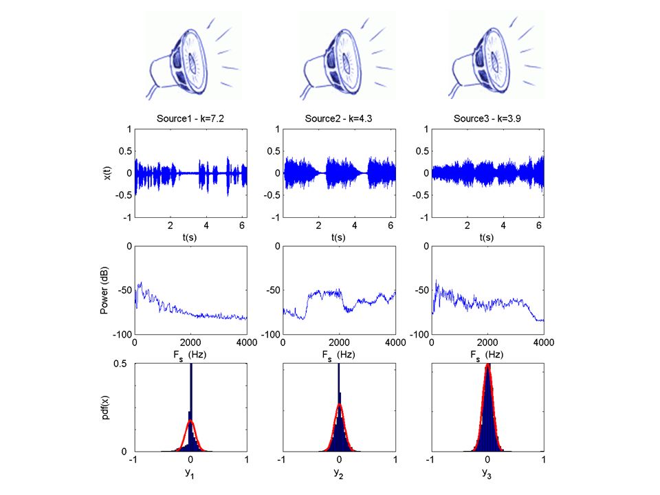
50. … some real examples using ICA The cocktail party problem revisited

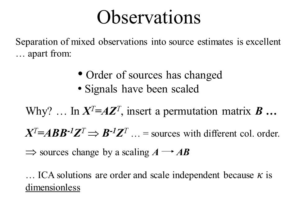
54. Why? … In X T =AZ T, insert a permutation matrix B … X T =ABB -1 Z T  B -1 Z T … = sources with different col. order.  sources change by a scaling A AB … ICA solutions are order and scale independent because κ is dimensionless Observations Separation of mixed observations into source estimates is excellent … apart from: Order of sources has changed Signals have been scaled

55. Separation of sources in the ECG

56.  =3  =11  =0  =3  =1  =5  =0  =1.5

57. Transformation inversion for filtering Problem - can never know if sources are really reflective of the actual source generators - no gold standard De-mixing might alter the clinical relevance of the ECG features Solution: Identify unwanted sources, set corresponding (p) columns in W -1 to zero (W p -1 ), then multiply back through to remove ‘noise’ sources and transform back into original observation space.

58. Transformation inversion for filtering

59. Real data X Y=WX Z X filt = W p -1 Y

60. ICA results 4 X Y=WX Z X filt = W p -1 Y

61. PCA is good for Gaussian noise separation ICA is good for non-Gaussian ‘noise’ separation PCs have obvious meaning - highest energy components ICA - derived sources : arbitrary scaling/inversion & ordering …. need energy-independent heuristic to identify signals / noise Order of ICs change - IC space is derived from the data. - PC space only changes if SNR changes. ICA assumes linear mixing matrix ICA assumes stationary mixing De-mixing performance is function of lead position ICA requires as many sensors (ECG leads) as sources Filtering - discard certain dimensions then invert transformation In-band noise can be removed - unlike Fourier! Summary

62. Fetal ECG lab preparation

63. Fetal abdominal recordings Maternal ECG is much larger in amplitude Maternal and fetal ECG overlap in time domain Maternal features are broader, but Fetal ECG is in-band of maternal ECG (they overlap in freq domain) 5 second window … Maternal HR=72 bpm / Fetal HR = 156bpm Maternal QRS Fetal QRS

64. MECG & FECG spectral properties Fetal QRS power region ECG Envelope Movement Artifact QRS Complex P & T Waves Muscle Noise Baseline Wander

65. Fetal / Maternal Mixture Maternal Noise Fetal

66. Appendix: Outlier insensitive ICA cost functions

67. In general we require a measure of statistical independence which we maximise between each of the N components. Non-Gaussianity is one approximation, but sensitive to small changes in the distribution tail. Other measures include: Measures of statistical independence I Mutual Information I, J Entropy (Negentropy, J )… and Maximum (Log) Likelihood (Note: all are related to  )

68. Entropy-based cost function Kurtosis is highly sensitive to small changes in distribution tails. A more robust measures of Gaussianity is based on differential entropy H(y), … negentropy: where y gauss is a Gaussian variable with the same covariance matrix as y. J(y) can be estimated from kurtosis … Entropy: measure of randomness- Gaussians are maximally random

69. Minimising Mutual Information Mutual information (MI) between M random variables: always non-negative and zero if variables are independent.  minimise MI. MI can be re-written in terms of negentropy … where c is a constant. differs from negentropy by a constant and a sign change I I = H x + H y - H xy

70. Generative latent variable modelling N observables, X... from N sources, z i through a linear mapping W=w ij Latent variables assumed to be independently distributed Find elements of W by gradient ascent - iterative update by where  is some learning rate (const) … and is our objective cost function, the log likelihood Independent source discovery using Maximum Likelihood

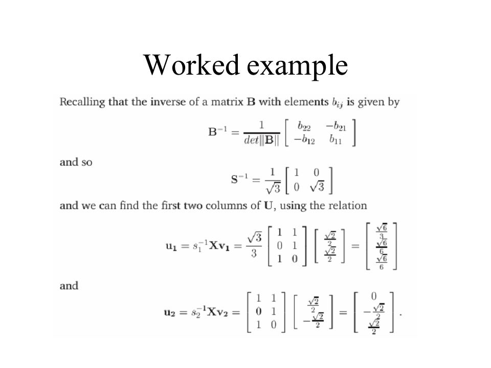
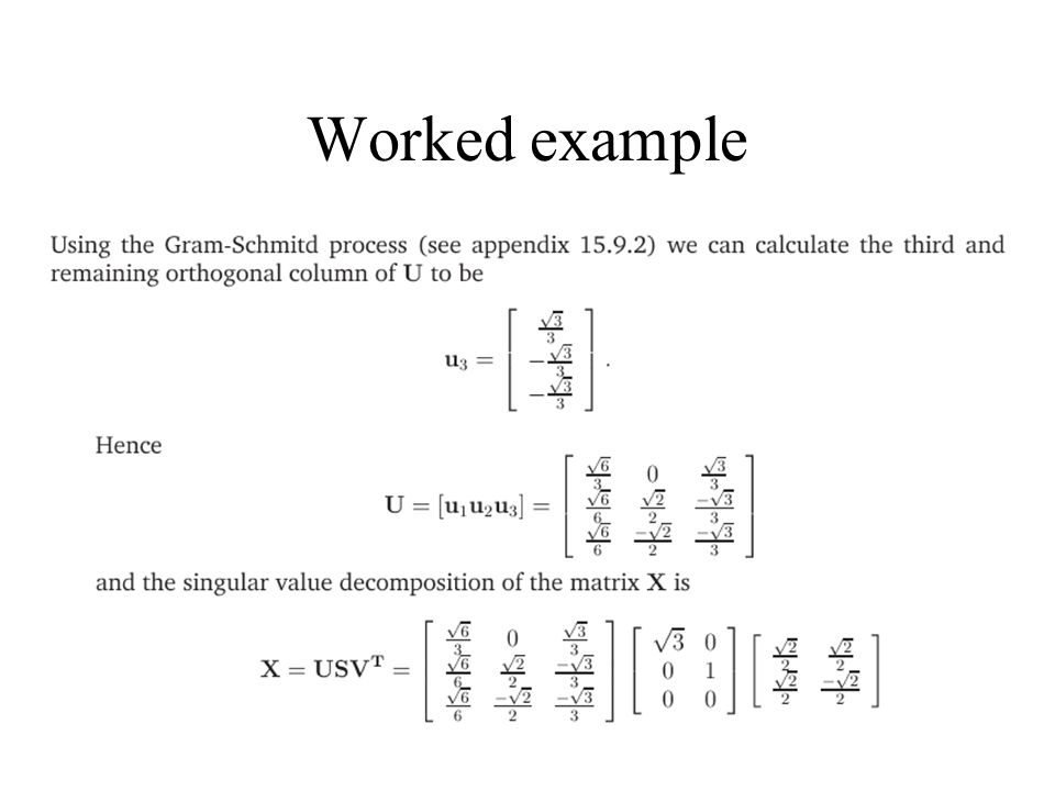
71. Appendix Worked example (see lecture notes)

72. Worked example