1. Radio Propagation - Mobile Radio Channel

2. Propagation - Mobile Radio Channel Difficult environment due to random, time-varying phenomena as a result of signal reflections, diffractions and scattering (multi-path), relative motion, shadowing. Main Impairments  Path loss - - attenuation with distance  Shadowing - - long-term variation of signal caused by (slow fading) obstructions (hills,buildings,mountain,foliage and for indoor wireless, walls, furniture  Multipath - - short-term signal variations due to multiple (fast fading) reflections from buildings, walls and ground.

3. Path loss Prediction of average received signal strength at a given distance from transmitter. Hundred to thousands meters → Large scale propagation model. Inverse power law

4. Path loss Reflections arise when the plane waves are incident upon a surface with dimension that are very large compared to the wavelength. Diffraction occurs according to Huygen’s principle when there is an obstruction between the transmitter and receiver antennas, and secondary waves are generated behind the obstructing bodies. Scattering occurs when the plane waves are incident upon an object whose dimensions are on the order of a wavelength or less, and causes the energy to be redirected in many directions.

5. Figure 4.1 Description of a mobile radio environment

6. Path loss Base to mobile link length is usually < 24 km. Path loss model not considering radio horizon effect (radio path loss attributable to curvature of earth) is available for distance up to 24 km.  Local scatterers surrounding the mobile cause short term or fast fading.  The radius of the active scatterer region at 850 MHz was found to be around 100 λ 2. The active scatterer region moves with the mobile as its centre. Some scatterers become inactive as the mobile drove away from them while some become active as the mobile approach them. When the operating frequency is lower, the propagation loss is smaller, the radius of the scatterer region becomes slightly larger.

7. Figure4.2 Schematic diagram of the propagation loss

8. Path loss Assume the receiver is moving at a constant speed V, distant r from transmitter is r =Vt. Variation of received signal strength or power with r can be viewed as variation with respect to time, t.

9. Path loss —— Mobile Radio Environment Propagation between base station and mobile unit not only by way of line of sight (LOS) route, but via many paths, by way of scattering, by reflections from or diffraction around buildings and terrain. Received signal by the mobile consists of a large number of plane waves whose amplitudes, phases, and angles of arrival relative to the direction of vehicle motion are random. These plane waves interfere and produce a varying field strength pattern with minima and maxima spaced on the order of a quarter wavelength. With the short wavelengths at the UHF and microwave frequencies, the received signal fades rapidly and deeply as the mobile moves through the interference pattern.

10. Path loss —— Multipath Typical mobile channels (outdoors and indoors), often there is no LOS path between transmitter and receiver. Received signal is the superposition of many (plane-wave) components of (approximately) equal power with random amplitude and phase that are independent. The resultant signal shows constructive (large amplitude) and destructive (small amplitude) patterns ⇒ time varying signal amplitude/ fading. Sum varies widely → 30 to 40 dB. Variability or rapid fluctuation of received signal strength in close proximity to a particular location or over very short travel distances (a few λ ) or short time durations (order of seconds) → small scale →fading model.

11. Path loss —— Multipath Figure4.3 Typical Profile of received signal’s Raleigh fading envelope and phase. Vehicular MS speed of 30mph,carrier frequency of 900MHz is information bearing phase, is random FM noise.

12. Mobile moving at a constant speed V. Difference in path lengths travelled by wave from remote source S to the mobile at points X and Y is ∆t is the time required for mobile to travel from X to Y, and is assumed to be the same at points X and Y since source is very far away. Doppler Shift

13. The phase change in the received signal due to the difference in path lengths is Where is the wave propagation constant. The apparent change in frequency or Doppler Shift is

14. Doppler Shift Mobile moving toward the direction of the arrival of the wave, Doppler Shift is positive, that is the apparent received frequency is increased. Mobile moving away from the direction of the arrival of the wave, Doppler shift is negative, that is the apparent received frequency is decreased. When, the Doppler shift is maximum. This leads to

15. Doppler Shift —— Example A transmitter radiates a CW of 1800 MHz. Calculate the maximum Doppler Shift experienced by a receiver on a vehicle moving at 100km/hr. Then compute the received carrier frequency if the mobile is moving (a) directly towards the transmitter, (b) at 90o to the direction of arrival of the transmitted wave and (c) at 30o to the direction of arrival of the transmitted wave.

16. Doppler Shift —— Example

17. Doppler Shift —— Transmission Coefficient T(t). Amplitude and phase of the received signal when a unit amplitude continuous wave (CW) signal is transmitted. Transmitted: Mobile travels in the x-direction with speed V. Vehicle motion introduces a Doppler Shift in every wave:

18. Doppler Shift —— Transmission Coefficient T(t). Assume the transmitted field is vertically polarized. The E field seen at the mobile is Rice’s model of narrowband gaussian noise

19. Doppler Shift —— Transmission Coefficient T(t). is random phase of the n-th arriving wave, distributed uniformly over( 0, 2 π). Received: Fading → Decreases in the magnitude of T( t ) with time as themobile moves through the interference pattern.

20. Doppler Shift —— Transmission Coefficient T(t). Variations in the phase of T( t ),,as time is varied →‘random FM’. Variations in the amplitude and phase of T( t ) → as the frequency is varied are called the frequency selective fading and phase distortion of the channel, respectively. (to be dealt with in a later section).

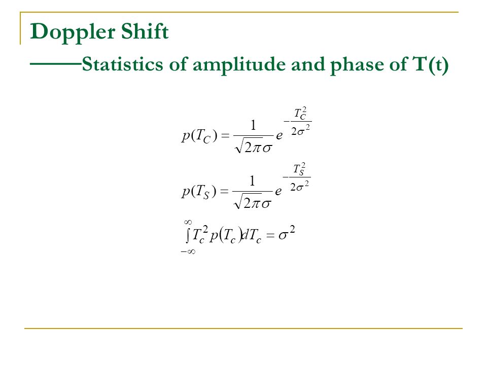
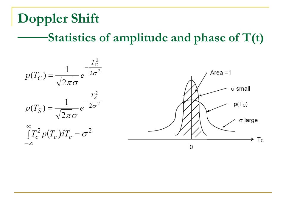
21. Doppler Shift —— Statistics of amplitude and phase of T(t) T(t) is a complex stochastic process. With a given transmitted frequency fc, T(t) is the result of many received plane waves, each shifted in frequency by the Doppler Shift appropriate to the vehicle motion relative to the direction of the plane wave. Thus, the received signal is the sum of a large number of sinusoids of comparative amplitude and random phase, whose frequencies are confined to the Doppler spread around fc. This received signal conforms to the Rice’s model of narrowband ‘Gaussian noise’.

22. Doppler Shift —— Statistics of amplitude and phase of T(t) For N sufficiently large, by central limit theorem, both TC(t) and TS(t) are zero mean Gaussian random processes. They are uncorrelated and independent with

23. Doppler Shift —— Statistics of amplitude and phase of T(t)

26. With Rayleigh pdf T c and T s are independent Gaussian random variables with zero means and variances.

27. Doppler Shift —— Statistics of amplitude and phase of T(t) Tc and Ts are independent because they are uncorellated. Their joint probability density is

28. Doppler Shift —— Statistics of amplitude and phase of T(t) → Rayleigh pdf

29. Doppler Shift —— Statistics of amplitude and phase of T(t) r and θ are independent random variables.

30. Doppler Shift —— Statistics of amplitude and phase of T(t) Variance of r,

31. Doppler Shift —— Correlation Functions of T(t)

32. Doppler Shift —— Statistics of amplitude and phase of T(t)

33. Doppler Shift —— Statistics of amplitude and phase of T(t) Consider as a wide sense stationary bandpass random process.

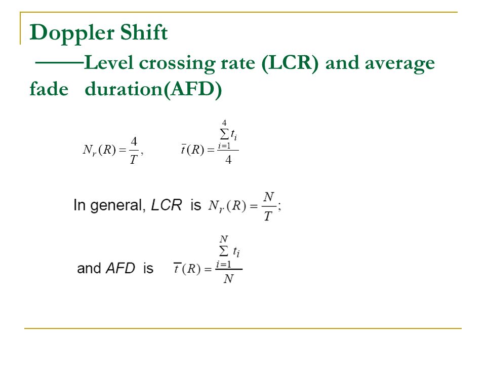
34. Doppler Shift —— Level crossing rate (LCR) and average fade duration(AFD)

36. Relates time rate of change, to level of received signal envelope, and to speed of mobile. Average number of level crossings per second at specified R

37. Doppler Shift —— Level crossing rate (LCR) and average fade duration(AFD)

38. N R is a function of mobile speed is apparent from the presence of f m in (1). Few crossings at both high and low level. N R is proportional to the product At high ρ, N R is small because of At low ρ, N R is small because of ρ.

39. Level Crossing Rates, N R Expected rate at which envelope, r, crosses a specified level, R. where the dot is time derivative and is the joint density function of r and at R = r. Rice gives

40. Level Crossing Rates, N R Integrating expression (2) over from 0 to 2π and from -∞ to +∞, we get Derivation of Probability Density Function Recall that

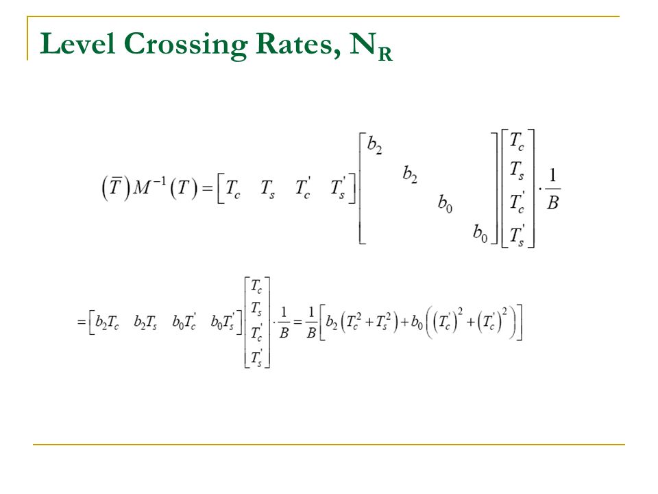
41. Level Crossing Rates, N R For N sufficiently large, by central limit theorem, both T C (t) and T S (t) are zero mean Gaussian random processes. For a fixed t, they are uncorrelated and independent zero mean Gaussian random variables with variance Now

42. Level Crossing Rates, N R For a fixed t, they are also uncorrelated and independent zero mean Gaussian random variables with variance. The joint pdf of multivariate Gaussian random variable is Where M is covariance matrix.

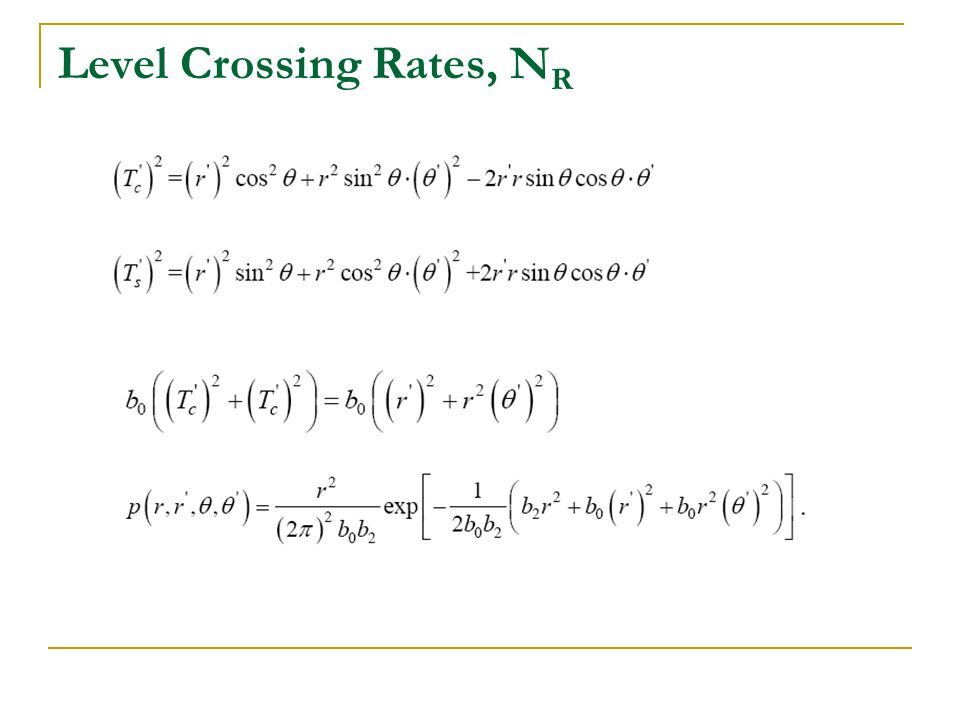
43. Level Crossing Rates, N R

46. Substituting (3) into (1) we get

47. Level Crossing Rates, N R Derivation of b 0

48. Level Crossing Rates, N R Derivation of b 2

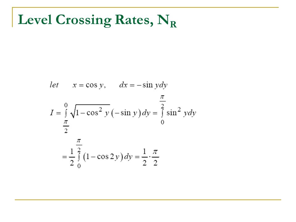
49. Level Crossing Rates, N R

51. Signal envelopes experience deep fades only occasionally, but shallow fades are frequent. Maximum number of level crossings occurs at 3dB below rms level.

52. Level Crossing Rates, N R Fig. Fading Rate:Level crossing rate of vertical monopole

53. Level Crossing Rates, N R —— Average duration of fade This is found by dividing the fading rate into the cumulative probability distribution: Fig. Average duration of fade

54. Level Crossing Rates, N R —— Average duration of fade

55. Level Crossing Rates, N R — Time Delay Spread and Coherence Bandwidth The results on fading derived so far are based on the assumption of a CW signal (un-modulated carrier) and that there is no difference between the arrival times of the multipath waves In fact, differences exist in the multi-path delays. Consider a CW being transmitted to a mobile unit.

56. Level Crossing Rates, N R — Time Delay Spread and Coherence Bandwidth

57. All scatterers associated with a certain path length can be located on an ellipse with the transmitter and receiver at its foci. TAR and TBR have the same arrival angle but different time delays. TBR and TCR have the same time delays but different angle of arrival. The received field is sum of a number of waves,

58. Level Crossing Rates, N R — Time Delay Spread and Coherence Bandwidth n th wave arriving at an angle composed of M waves with propagation delay times T nm. All these M waves experience the same Doppler shift, f n is maximum when Note that actually the argument of each cosine term in (1) should be

59. Level Crossing Rates, N R — Time Delay Spread and Coherence Bandwidth Since Here, C nm is determined from which is fraction of the incoming power within d α of the angle α and within dT of the delay T, in the limit with N and M very large.

60. Level Crossing Rates, N R — Time Delay Spread and Coherence Bandwidth Now consider propagation of signal that occupies a finite bandwidth. Consider two frequency components within the signal bandwidth. If the frequencies are close together, then the different propagation paths will have approximately the same electrical length for both components. Their amplitude and phase variations will be very similar. Provided the signal bandwidth is sufficiently small, all frequency components within it behave similarly and flat fading is said to exist.

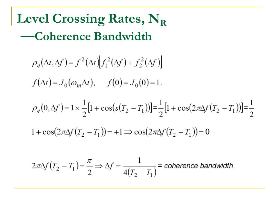
61. Level Crossing Rates, N R — Time Delay Spread and Coherence Bandwidth If the frequency separation is large enough, the behavior at one frequency tends to become uncorrelated with or independent from that at the other frequency, because the phase shifts along the various paths are different at the two frequencies. The maximum frequency difference for which the CW’s are still strongly correlated is called the ‘coherence bandwidth’ of the mobile transmission channel. Coherence Bandwidth is proportional to the inverse of the delay spread or the magnitude of the difference between the delay times.

62. Level Crossing Rates, N R — Time Delay Spread and Coherence Bandwidth Typical spreads in time delays range from a fraction of a µ-seconds to many µ-seconds. Longer spreads in urban and shorter spreads in suburban areas. Signals that occupy a bandwidth greater than the coherence bandwidth will become distorted since the amplitudes and phases of the various spectral components in the received signal are not the same as they were in the transmitted signal. ⇒ Frequency selective fading.

63. Level Crossing Rates, N R — Envelope Correlation Function or Envelope Correlation Coefficient In this section, we are interested to derive the Envelope Correlation Function or Envelope Correlation Coefficient between two CW’s as a function of frequency separation and time separation. Two CW’s at ω1 and ω2,

64. Level Crossing Rates, N R — Envelope Correlation Function or Envelope Correlation Coefficient For large enough N and M, xi(t) ‘s are Gaussian random processes. (By Central Limit Theorem).

65. Level Crossing Rates, N R — Envelope Correlation Function or Envelope Correlation Coefficient Now we are interested in the correlation of the envelope of the CW’s as a function of both time separation, ∆t, and frequency separation, Define, for fixed t, These r.v. can also be written in terms of their envelopes and phases,

66. Level Crossing Rates, N R — Envelope Correlation Function or Envelope Correlation Coefficient Moments of the r.v.’s, The average will vanish unless n=p and m=q, which gives

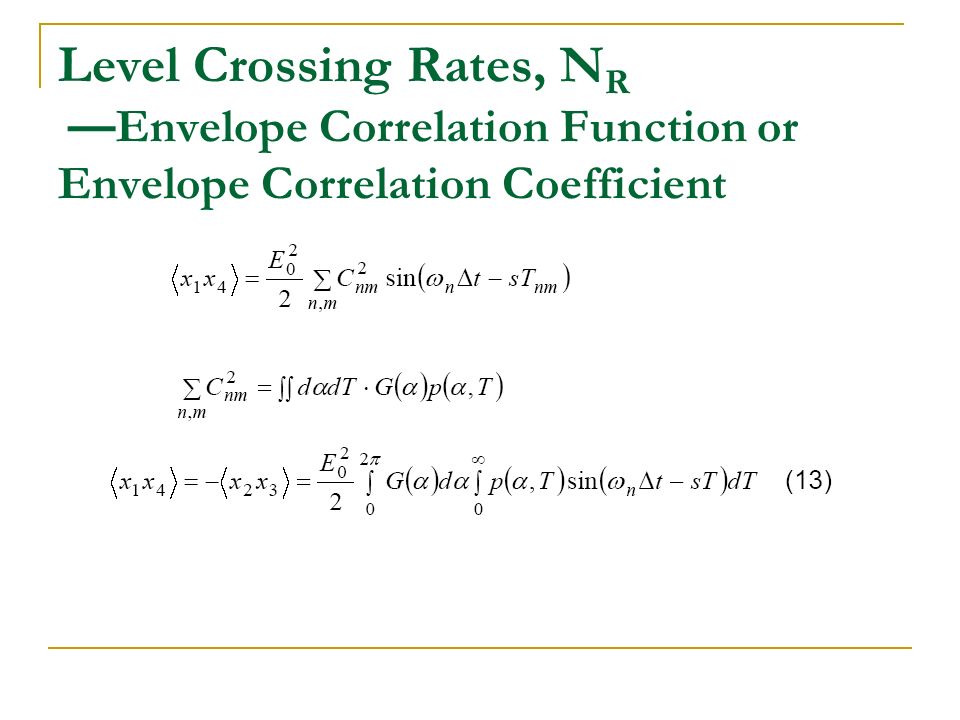
67. Level Crossing Rates, N R — Envelope Correlation Function or Envelope Correlation Coefficient In the limit as N, M → ∞: By similar arguments

68. Level Crossing Rates, N R — Envelope Correlation Function or Envelope Correlation Coefficient

70. Recall Similarly,

71. Level Crossing Rates, N R — Envelope Correlation Function or Envelope Correlation Coefficient Now these moments are parameters in the joint pdf of Transforming the rv’s to the amplitudes and phases, we get the corresponding pdf in terms of and.

72. Level Crossing Rates, N R — Envelope Correlation Function or Envelope Correlation Coefficient Where Now assume an exponential distribution of the delay spreads and a uniform distribution in angle of the incident power.

73. Level Crossing Rates, N R — Envelope Correlation Function or Envelope Correlation Coefficient Assume also that. The quantities in (17) may be worked out with the help of (10) to (15). Equation (15),

74. Level Crossing Rates, N R — Envelope Correlation Function or Envelope Correlation Coefficient

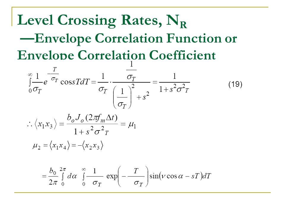
76. Using integration by parts on (19), can show that In summary, (21)

77. Level Crossing Rates, N R — Envelope correlation coefficient

78. where

79. Level Crossing Rates, N R — Frequency Selective Fading Two CW’s separated by a finite frequency range, propagating in a medium, do not observe the same fading. Frequency selective fading is closely related to the time delay spread,. Considering correlation in two frequencies but no time or space separation. That is

80. Level Crossing Rates, N R — Frequency Selective Fading Let as a criterion for determining the coherence bandwidth, we have from (27), (28) Coherence bandwidth is inversely proportional to time delay spread.

81. Level Crossing Rates, N R — Frequency Selective Fading Open areas: Suburban areas: Urban areas:

82. Level Crossing Rates, N R — Coherence Time Letting ∆f =0,we have from (27) Again using as a criterion for correlatedness in time, we have

83. Level Crossing Rates, N R — Coherence Time

84. Level Crossing Rates, N R — Spatial correlation of the envelope Many mobile radio systems employ antenna diversity, where spatially separated antennas provide multiple faded replicas of the same information-bearing signal. What should be the antenna separation to provide uncorrelated antenna diversity branches? Consider two places separated by d. The mobile receiver is moving at speed V. The correlation function in terms of ∆t is equivalent to that in terms of the distance d = Vt.

85. Level Crossing Rates, N R — Spatial correlation of the envelope Assuming a uniform and noting that, we have The auto-covariance is zero at 0.38λ, and is less than 0.3 for As a rule of thumb, uncorrelated diversity branches can be obtained at the mobile station by placing the antenna elements about a half wavelength apart.

86. Level Crossing Rates, N R — Spatial correlation of the envelope Base station space diversity Figure 4.5 Analytical model for spatical correlation at a base station

87. Level Crossing Rates, N R — Spatial correlation of the envelope The above result cannot usually be applied to a base station, since the uniform arrival angle is hardly satisfied. Because of the height of the base station antenna, there are few scattering objects around the base station. Since the arrival angle is not uniformly distributed, and the range of the arrival angle, correspondingly, the spread of the Doppler frequencies becomes smaller. Therefore, the time or spatial correlation at a base station becomes broad. (Recall that autocorrelation function is Fourier Transform of power spectrum).

88. Level Crossing Rates, N R — Spatial correlation of the envelope A spatial separation of the order of 10 λ is required for a base station diversity system. The fact that the active scatterers are moving with the mobile while the base station is standing still, can be viewed equivalently, as the active scatterers are standing still while the base station is moving at a speed V.

89. Level Crossing Rates, N R — Coherence Bandwidth and Power Delay Profile In the derivation of the envelope correlation coefficient,it is assumed that the wave arrival angle and path delay are statistically independent. That is This assumption makes it possible to express both µ 1 and µ 2 as the product of a function of ∆f only and a function of ∆t only. That is

90. Level Crossing Rates, N R — Coherence Bandwidth and Power Delay Profile where

91. Level Crossing Rates, N R — Coherence Bandwidth and Power Delay Profile Similarly Now

92. Level Crossing Rates, N R — Coherence Bandwidth and Power Delay Profile

93. Exercise: Find an expression for the coherence bandwidth of a mobile radio channel modelled by a two- path power delay profile:

94. Level Crossing Rates, N R — Coherence Bandwidth

96. Rician Distribution Rayleigh fading model is suitable for urban areas where high-rise building often block the line of sight (LOS) path between transmitter and receiver. When a LOS exists in addition to the multipath waves from scatterers → Rician Fading Model. → Suburban areas, micro or pico-cellular.

97. Rician Distribution Received signal y(t):

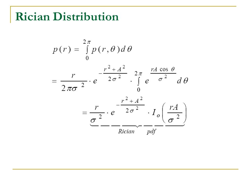
98. Rician Distribution

99. Rician Distribution

101. Modified Bessel function of the first kind and order zero. For A=0, I 0 (0) = 1, p(r) above reduces to the Rayleigh pdf. The pdf of the phase θ is given by

102. Rician Distribution

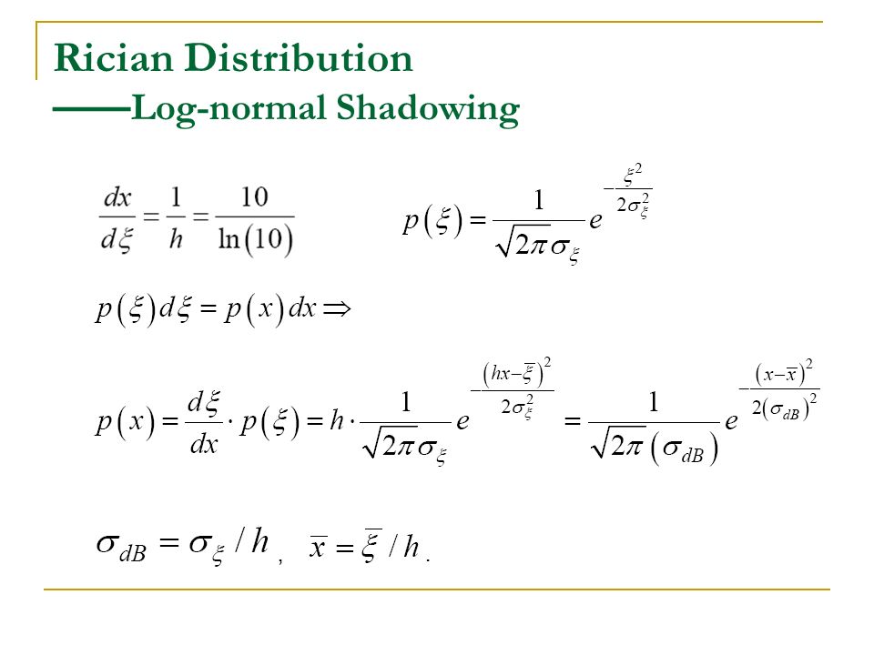
103. Rician Distribution —— Log-normal Shadowing Random shadowing effects which happen over a large number of measurement locations which have the same Transmitter-Receiver (T-R) separation but different level of clutter along the propagation path. Local mean signal strength (that is, the signal strength averaged over the Rayleigh fading) in an area at a fixed radius from a particular base station antenna is log- normally distributed. The received power at a mobile at distance d is

104. Rician Distribution —— Log-normal Shadowing r is a Rayleigh distributed r.v., e ξ accounts for the shadowing ( ξ isGaussian with zero mean and variance ), Kd −η is the deterministic loss law, and P T is the transmitter power. Averaging the received signal strength over the Rayleigh fading, we get

105. Rician Distribution —— Log-normal Shadowing

107. Example: The local mean signal strength in areas at a fixed radius from a particular base station is log-normally distributed. Suppose the mean value of this local mean signal strength is 5 dBm and that the standard deviation is 6 dB. What is the particular local mean signal level, γ dB, so that the probability of it being exceeded is 10%? Solution:

108. Rician Distribution —— Log-normal Shadowing

109. Time-delay Spread – modulation effects The concepts of time delay spread and coherence bandwidth have been dealt with in the last Section for CW signals only, that is without considering the effect of modulation. Now we consider modulation effects. Multipath channel causes delayed “echoes” of the transmitted signal, each with Rayleigh amplitude and uniform phase. If these delays are such that their spread is a significant fraction (>50%) of the symbol duration [or exceeds symbol duration] ⇒ smearing of the transmitted signal, i.e. Inter-Symbol Interference (ISI).

110. Time-Delay Measurements

111. Delay Spread Function h(t, τ) Transmitted signal x(t) complex envelope or low-pass equivalent signal ⇒ containing the modulation. Received waveform from paths with delay This is already the result of superposition of many waves coming fromall directions, but with delays of the order of grouped together.

112. Delay Spread Function h(t, τ) Note that and are random processes, which means that the effect of Doppler spread is already included. Relate The received signal is then where For a large number of paths, can consider the received signal as a continuum of multipath components.

113. Delay Spread Function h(t, τ) all between and are grouped together.

114. Delay Spread Function h(t, τ) → Delay Spread function or Impulse Response of channel.

115. Delay Spread Function h(t, τ) → Since For a linear time invariant system h(t) : Channel response to a impulse at t = 0.

116. Delay Spread Function h(t, τ) For a time-variant channel, the response to an impulse applied at t =ζ will not have the same shape as the response to an impulse applied at t = 0. Introduce : channel response for an impulse applied at t =ζ, From (2), instead of we have, therefore

117. Delay Spread Function h(t, τ) now let Recalling from (1) that we have : Channel response at t to an impulse applied at time t - τ,that is applied at τ seconds in the past.

118. Delay Spread Function h(t, τ)

120. Fig. Examples of random channel impulse response in two dimensions (a) time-variant channel

121. Delay Spread Function h(t, τ) Fig. Examples of random channel impulse response in two dimensions (b) time-invariant channel

122. Delay Spread Function h(t, τ) —— Channel Classification In this section since we have included modulation in the analysis, we can relate B c and T c to B s and f m. Frequency flat, multiplicative (time selective fading). B s << B c, where, B s = signal bandwidth, B c = coherence bandwidth.

123. Delay Spread Function h(t, τ) —— Channel Classification All frequency components in U(f) undergo the same attenuation and linear phase shift through the channel. since U(f) has its frequency content concentratedin the vicinity of f = 0.

124. Delay Spread Function h(t, τ) —— Channel Classification If rate of change of a s (t ) with t is smaller than rate of change of u(t) with t, then shape of signal pulse is preserved. However it undergoes amplitude fading whenever dips. Frequency selective, time flat channels. Received signal duration (time during which signal is in flight) less than coherence time. T s < T c → Channel appears to the signal as time invariant. → Time flat channels.

125. Delay Spread Function h(t, τ) —— Channel Classification However frequency selectivity means B s > B c,which implies that the signal spectrum U(f) will be modified by the multiplication with H(f). Shape of received waveform distorted. Also for digital transmission, Inter-Symbol-Interference (ISI).

126. Delay Spread Function h(t, τ) —— Classification of Multi-path Fading 2 Channel parameters (1) Multi-path (rms) spread / coherence BW captures the multi-path channel conditions via delay- spread (in-time) or amplitude correlation (in frequency).

127. Delay Spread Function h(t, τ) —— Classification of Multi-path Fading (2) Doppler spread / Coherence Time captures the rate of multi-path channel variations via spread of carrier (in frequency) or correlation of channel impulse response (in time).

128. Delay Spread Function h(t, τ) —— Two System Design Parameters (1) Symbol Period: Ts (2) Transmission BW: Bs Narrowband (PSK / QAM) : Wideband (Spread - Spectrum)

129. Delay Spread Function h(t, τ) —— Classification Based on Multipath Spread Flat (Freq. Non-select Fading) : Freq.-Select Fading Transmitted pulse shape is : Transmitted pulse shape (relatively) undisturbed, but : is distorted. amplitude fades with time :

130. Delay Spread Function h(t, τ) —— For Narrowband Modulation ∴ Flat Fading ←→ No Inter-symbol Interference (ISI). Frequency Selective Fading

131. Delay Spread Function h(t, τ) —— For Wideband Modulation Suppose (no ISI) However, it is possible that But ， Frequency-Selectivity. For wide-band signals, possible to have no ISI and frequency selectivity simultaneously.

132. Delay Spread Function h(t, τ) —— Classification Based on Doppler Spread Fast Fading : Slow Fading Large Doppler Spread : Small Doppler Spread ⇒ Channel variations : ⇒ Channel variation slower faster than baseband : than baseband signal variation signal, variations. : channel is approximately invariant : over several symbol duration.