1. Fossen Chapter 2 Deformation

2. Components of deformation, displacement field, and particle paths

3. Displacement (D): Vector connecting the initial and final positions of a deformed particleX2
Final position
(x’1, x’2)
x’2 = x2 + v
Particle path v D x2
(x1, x2) u
Initial position x1
x’1 = x1 + u X1

4. Deformation Matrix
|D11 D12 D13|
Dij= |D21 D22 D23|
|D31 D32 D33|
The matrix (vector processor), transforms the position vector of each point
Like the wind, that transforms the vector (direction) of a boat!
Linear Transformation: x’=Dx or x=D-1x’
For example: X’1=D11x1+D12x2+D13x3
|x’1| = |D11 D12 D13| |x1|
|x’2| = |D21 D22 D23| |x2|
|x’3| = |D31 D32 D33| |x3|

5. Nine quantities needed to define the homogeneous strain matrix
|e11 e12 e13|
|e21 e22 e23|
|e31 e32 e33|
eij , for i=j, represent changes in length of 3 initially perpendicular lines
eij , for ij, represent changes in angles between lines

6. Total deformation of an object (a) displacement vectors connecting initial to final particle position (b)-(e) – particle paths (b), (c) Displacement field

7. Homogeneous deformation
Straight lines remain straight
Parallel lines remain parallel
Linear transformation
Pure and simple shear deformation of brachiopods, ammonites, and dikes

8. Homogeneity depends on scale
The overall strain is heterogeneous.
In some domains (segments), strain is homogeneous

9. Discrete or discontinuous deformation can be viewed as continuous or homogeneous depending on the scale of observation
At large scale deformation seems to be homogeneous
At small scale, the discontinuities are more apparent, and it is inhomogeneous

10. Extension by faulting  is the same as stretch (S) for extensional basins!

11. Shear Strain Shear strain (angular strain) g = tan 
A measure of the change in angle between two lines which were originally perpendicular. Like e, g is dimensionless!
small change in angle is angular shear or 
Original circle of radius 1
Strain ellipse

12. Angular shear strain g is the change in angle between two initially perpendicular lines A & B
CW is +
CCW is -

14. Rotation of lines
Pure Shear
No change to the lines that originally parallel the
principal strain axes (white lines)

15. Perpendicular lines that are originally parallel to the incremental principal axes of strain, will remain perpendicular after strain

18. Rotational and Irrotational Strain
If the strain axes have the same orientation in the deformed and undeformed state we describe the strain as a non-rotational (irrotational) strain
If the strain axes end up in a rotated position, then the strain is rotational

19. Examples
An example of a non-rotational strain is pure shear - it's a pure strain with no dilation of the area of the plane
An example of a rotational strain is a simple shear

20. SIMPLE SHEAR: Constant volume, non-coaxial, plane strain (i.e., is 2D)
Involves a change in orientation of material lines along two of the principal axes (here: 1 and 2 )
SIMPLE SHEAR: Constant volume, non-coaxial, plane strain (i.e., is 2D)
i.e., ez=e3 = 0 across the page!
Has two circular sections: xz (slip plane) and yz (height)
Lines parallel to the principal axes rotate with progressive deformation
Deformation matrix (triangular)
| 1 g|
| 0 1| where g=tan  is the shear strain
Note: no change of length along x or y!
PURE SHEAR: Constant volume, coaxial, plane strain (i.e., is 2D)
Shortening in one direction (ky) is balanced by extension in the other (kx)
Deformation matrix (diagonal)
|Kx 0 |
|0 ky | where ky = 1/kx
Kx = S1=2/1) = 2
Ky = S2=0.5/1=0.5

21. Coaxial Strain
The infinitesimal principal axes are parallel in all increments!
second increment
initial state
Undeformed
first increment

22. Non-coaxial Strain incremental strain axes rotate
The infinitesimal principal axes rotate during each increment!
initial state
undeformed
first increment
second increment
third increment

23. Equation for the Strain Ellipsoid
The equation for an ellipsoid is: x2/a2 + y2/b2 + z2/c2 = 1 where a, b, c are semi-principal axes from the origin to the surface of the ellipsoid. These semi-principal axes for strain ellipsoid are the principal stretches S1, S2 and S3 x2/S12 + y2/S22 + z2/S32 = 1 Given: S12= 1 S22 = 2 S32 = 3 Substituting  for S, we get the equation for the strain ellipsoid in terms of : x2/1 + y2/2 + z2/3 = 1

24. Classification of strain ellipse in 2D Only Field 2 is used since XY
Field 1: e1 >0 & e2 >0
Classification of strain ellipse in 2D Only Field 2 is used since XY
e1= e2
e1 >0
e2 <0
= S2 = 1+e2
Field 3: e1 <0 & e2 <0
No ellipse here
1+e1 = 1+ e2 =1  e1=e2 = 0 A
1+e2 =1
1+e1=1
= S1 = 1+e1

25. Graphic representation of strain ellipse
Point A (1,1) represents an undeformed circle (1 = 2 = 1)
Because by definition, 1>2 , all strain ellipses fall below or on a line of unit slope drawn through the origin
All dilations fall on the 1 = 2 line through the origin
All other strain ellipses fall into one of three fields:
Above the 2=1 line where both principal extensions are +
To the left of the 1=1 where both principal extensions are –
Between two fields where one is (+) and the other (-)

26. Shapes of the Strain Ellipse

27. special case in this field S1S3 < 1.0
plane strain (S1S3 = 1.0) is
special case in this field
S1S3 < 1.0
S1=3
from: Davis and Reynolds, 1996

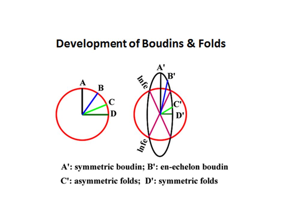
28. Structures depend on the orientation of the layer relative to the principal stretches and value of s2

29. Flinn Diagram b=Y/Z=1 Y=Z b=1 k= =1+e1/1+e2 a=1  k=0 a=X/Y=1  X=Y

30. k = (a-1)/(b-1)
Prolate (linear)
Isotropic
Oblate (tabular)

31. a. Flinn diagram b. Hsu diagram

32. Volumetric Strain (Dilation)
Gives the change of volume compared with its original volume
Given the original volume is vo, and the final volume is v´, then the volumetric stain, ev is:
ev =(v´-vo)/vo = v/vo [no dimension]

33. Volume change on Flinn Diagram
Recall: S=1+e = l’/lo and ev = v/vo =(v’-vo)/vo
An original cube of sides 1 (i.e., lo=1), gives vo=1
Since stretch S=l’/lo, and lo=1, then S=l’/1=l’
The deformed volume is therefore: v'=l’. l’. l’ = S.S.S
Orienting the cube along the principal axes
V' =S1.S2.S3 = (1+e1)(1+e2)(1+e3)
Since v =(v’-vo), for an original cube of vo=1, we get:
Volume change: v =v’-1 = (1+e1)(1+e2)(1+e3)-1

34. Dilation lo=x=1 S1=X=l’/lo=l’ lo=y=1 S2=Y=l’/lo=l’ lo=z=1
S3=Z=l’/lo=l’
Vo = 1
V' = l’.l’.l’ = S1.S2.S3 = (1+e1)(1+e2)(1+e3)
Volume change: v =v’-1 = (1+e1)(1+e2)(1+e3)-1

35. Given vo=1, since ev = v/vo, then ev = v =(1+e1)(1+e2)(1+e3) -1
1+ev =(1+e1)(1+e2)(1+e3)
If volumetric strain, v = ev = 0 then for no volume change
(1+e1)(1+e2)(1+e3) = 1 i.e., XYZ=1
Let’s take natural log of 1+ev =(1+e1)(1+e2)(1+e3):
ln(1+ev) = e1+e2+e3 (note: ln 1 = 0)
Rearrange: (e1-e2)=(e2-e3)-3e2+ln(1+ev)
Plane strain (e2=0) leads to: (e1-e2)=(e2-e3)+ln(1+ev)
which is the same as: ln X/Y= ln Y/Z + ln (1+ev)
This is the equation of a straight line (y=mx+b) on a log-log plot of ln X/Y vs. ln Y/Z, with a slope, m=1
See next slide!

36. Ramsay Diagram ln X/Y= ln Y/Z + ln (1+ev) Y = Kx + b (K is the slope)
When there is no volume change (ev= 0), the straight line goes through the origin.
For + ev, the straight line shifts to the left
For - ev, the straight line shifts to the right

37. Ramsay Diagram (previous slide)
Small strains are located near the origin
Equal increments of progressive strain (i.e., strain path) plot along straight lines
Unequal increments plot as curved plots
If v=ev is the volumetric strain, then:
1+v =(1+e1)(1+e2)(1+e3)  = lnS = ln(1+e)
It is easier to examine v on this plot Take log from both sides and substitute  for ln(1+e)
ln(v +1)= 1+ 2+ 3
If v>0, the lines intersect the ordinate
If v<0, the lines intersect the abscissa

38. Compaction involves strain (can be viewed as shrinkage and strain
Compaction involves strain (can be viewed as shrinkage and strain. The order is not important. Final strain ellipses for the three cases are the same!
Coaxial deformation

39. States of strain: Uniaxial, planar, and 3D General Strain: Involves extension or shortening in each of the principal directions of strain 1 > 2 > 3 all  1 X Z Z Y Z
shortening along Z compensated with equal extension along Y and Z
e2 = 0 Y
Extension along X compensated with equal shortening along Y and Z X X Z X Z Y Y
shortening along Z compensated with equal extension along Y and Z
Strain ellipse: Prolate spheroid or cigar shaped
Strain ellipse:oblate spheroid or pancake shaped

40. The strain ellipsoid Note: error on the figure of the book’s module
The strain ellipsoid Note: error on the figure of the book’s module! |1+e1|= X=S1 |1+e2|= Y=S2 |1+e3|= Z=S3

41. Strain ellipse

42. Isotropic volume change (involves no strains)
Anisotropic volume change by uniaxial shortening (compaction)
 is the elongation
In the vertical direction.
1+  is the vertical stretch.
i.e., change is only in one direction.
Strain ellipse is oblate (pancake).
Isotropic volume increase: X = Y = Z > 1
Isotropic volume decrease: X = Y = Z < 1

43. Compaction (uniaxial strain) reduces the dips of both layers and fault

44. Simple shear and shear direction refer to the more general type of deformation such as the subsimple shear
There is a spectrum of planar deformation between pure shear and
Simple shear , commonly referred to as subsimple shear (general shear).
It is a mixture of pure and simple shear.

45. Flow pattern: the sum of particle paths in a deforming medium
The most important deformation parameters: Boundary conditions control the flow parameters, which over time produce strain Flow paths are usually curved. When they are straight (i.e., when parallel the eigenvectors of defor. Matrix) , they are called flow apophyses (asymptotes) which separate different domains of particle paths (i.e., compartmentalize the flow patterns). In 3D, there are 1 to 3 possible apophyses. Particle located along the apophyses move straight; other move along curved paths. No particle cross a flow apophyses unless conditions change during deformation.
ISA1 and ISA3 are directions of max and min stretching at any instant of time during deformation.

46. Vorticity vector (w) in progressive subsimple shear
Vorticity vecto (w) during sub-simple shear
Vorticity: Internal rotation of particle lines w.r.t. the principal strain axes. It is a measure of coaxiality!
The vorticity vector (w) is always perpendicular to the shear direction, parallel to the shear plane.

47. Particle paths (green) and flow apophyses (blue) describing flow patterns for planar deformations. Apophyses: two orthogonal (parallel to strain axes) for pure shear; two oblique (non-orthogonal) for subsimple shear; and one coincident for simple shear
Simple shear: Only one apophsis. II SZB (shear zone boundary), Wk = 1. ISA at 45o to SZB. LNIE II and  to SZB
Kinematic vorticity (wk) number is the ratio of rotation rate (radian/s) and distortion rate (e/t).
Wk= zero for pure shear
 = 2/tan 
Coaxial flow: finite and instantaneous strain axes and apophyses coincide. Vorticity is zero.
Non-coaxial flow: the stran axes and rock particles rotate relative to each other.

49. Progressive strain during simple shear and pure shear
strain axes do not remain along the same material lines at different increments
Strain axes do not rotate relative to the material lines.

50. Simple shearing of three sets of orthogonal lines

51. Lines in the contraction and extension fields experience a history of contraction and extension, respectively.

52. Pure shearing of three sets of orthogonal lines

53. Subsimple shearing of three sets of orthogonal lines

54. Restored and current profile across the North Sea rift
Restored and current profile across the North Sea rift. Locally, it is modeled as simple shear, but is better treated as pure shear on larger scale