2. Chapter 13 Discrete Image Transforms
13.1 Introduction
13.2 Linear transformations
One-dimensional discrete linear transformations
Definition. If x is an N-by-1 vector and T is an N-by-N matrix, then is a linear transformation of the vector x, I.e.,
T is called the kernel matrix of the transformation

3. Linear Transformations
Rotation and scaling are examples of linear transformations
If T is a nonsingular matrix, the inverse linear transformation is

4. Linear Transformations
Unitary Transforms
If the kernel matrix of a linear system is a unitary matrix, the linear system is called a unitary transformation.
A matrix T is unitary if
If T is unitary and real, then T is an orthogonal matrix.

5. Unitary Transforms
The rows ( also the columns ) of an orthogonal matrix are a set of orthogonal vectors.
One-dimensional DFT is an example of a unitary transform or
where the matrix W is a unitary matrix.

6. Unitary Transforms Interpretation
The rows (or columns) of a unitary matrix form a orthonormal basis for the N-dimensional vector space.
A unitary transform can be viewed as a coordinate transformation, rotating the vector in N-space without changing its length.
A unitary linear transformation converts a N-dimensional vector to a N-dimensional vector of transform coefficients, each of which is computed as the inner product of the input vector x with one of the rows of the transform matrix T.
The forward transformation is referred to as analysis, and the backward transformation is referred to as synthesis.

7. Two-dimensional discrete linear transformations
A two-dimensional linear transformation is
where forms an N2-by-N2 block matrix having N-by-N blocks, each of which is an N-by-N matrix
If , the transformation is called separable.

8. 2-D separable symmetric unitary transforms
If , the transformation is symmetric,
The inverse transform is
Example: The two-dimensional DFT

9. Orthogonal transformations
If the matrix T is real, the linear transformation is called an orthogonal transformation. Its inverse transformation is
If T is a symmetric matrix, the forward and inverse transformation are identical,

10. Basis functions and basis images
The rows of a unitary form a orthonormal basis for a N-dimensional vector space. There are different unitary transformations with different choice of basis vectors. A unitary transformation corresponds to a rotation of a vector in a N-dimensional (N2 for two-dimensional case) vector space.

11. Basis Images
The inverse unitary transform an be viewed as the weighted sum of N2 basis image, which is the inverse transformation of a matrix as
This means that each basis image is the outer product of two rows of the transform matrix.
Any image can be decomposed into a set of basis image by the forward transformation, and the inverse transformation reconstitute the image by summing the basis images.

12. 13.4 Sinusoidal Transforms
The discrete Fourier transform
The forward and inverse DFT’s are
where

13. 13.4 Sinusoidal Transforms
The spectrum vector
The frequency corresponding to the ith element of F is
The frequency components are arranged as 1 i
N/2
N-1

14. 13.4 Sinusoidal Transforms
The frequencies are symmetric about the highest frequency component. Using a circular right shift by the amount N/2, we can place the zero-frequency at N/2 and frequency increases in both directions from there. The Nyquist frequency (the highest frequency) at F0. This can be done by changing the signs of the odd-numbered elements of f(x) prior to computing the DFT. This is because

15. 13.4 Sinusoidal Transforms
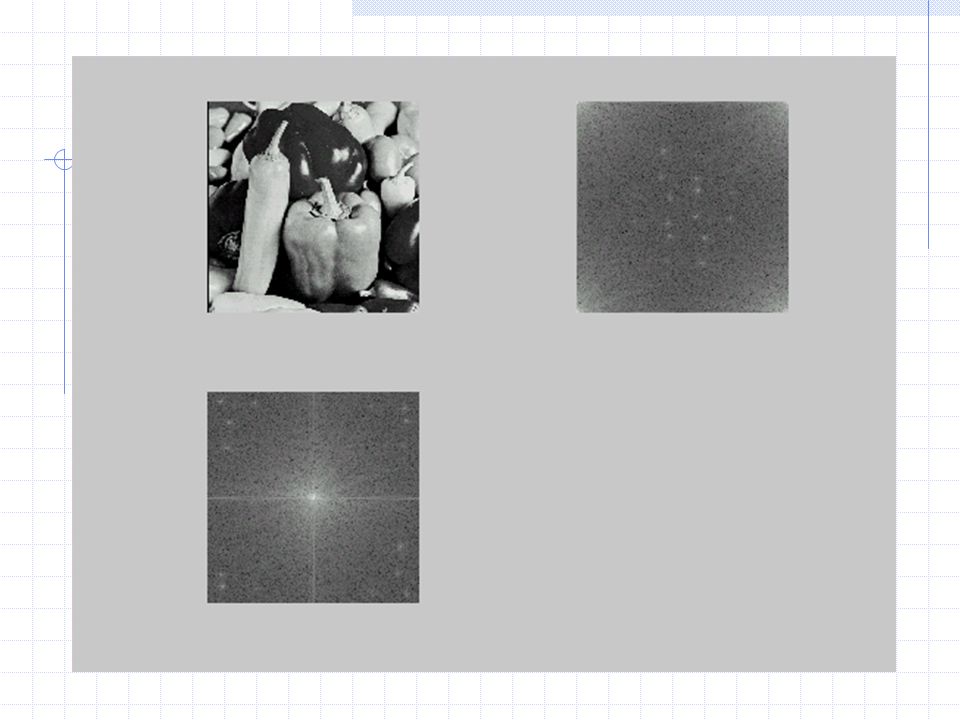
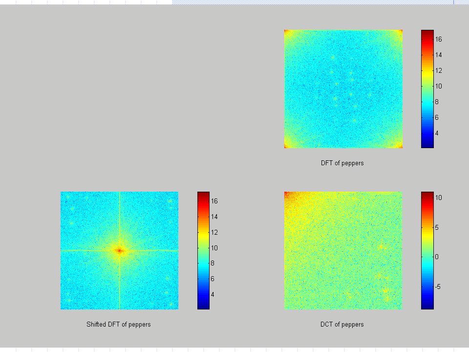
The two-dimensional DFT
For the two-dimensional DFT, changing the sign of half the elements of the image matrix shifts its zero frequency component to the center of the spectrum 1 4 3 2 2 3 4 1

17. 13.4.2 Discrete Cosine Transform
The two-dimensional discrete cosine transform (DCT) is defined as
and its inverse
where

18. The discrete cosine transform
DCT can be expressed as a unitary matrix form
Where the kernel matrix has elements
The DCT is useful in image compression.

20. The sine transform The discrete sine transform (DST) is defined as and
The DST has unitary kernel

21. The Hartley transform
The forward two-dimensional discrete Hartley transform
The inverse DHT
where the basis function

22. The Hartley transform
The unitary kernel matrix of the Hartley transform has elements
The Hartley transform is the real part minus the imaginary part of the corresponding Fourier transform, and the Fourier transform is the even part minus j times the odd part of the Hartley transform.

23. 13.5 Rectangular wave transforms
The Hadamard Transform
Also called the Walsh transform.
The Hadamard transform is a symmetric, separable orthogonal transformation that has only +1 and –1 as elements in its kernel matrix. It exists only for
For the two-by-two case
And for general cases

24. The Hadamard Transform
Ordered Hadamard transform

25. The Slant Transform
The orthogonal kernel matrix for the slant transform is obtained iteratively as

26. 13.5.3 The Slant Transform And
where I is the identity matrix of order N/2-2 and

27. The Slant Transform
The basis function for N=8 4 5 1 2 6 3 7

28. 13.5.4 The Haar Transform The Basis functions of Haar transform
For any integer , let
where and is the largest power of 2 that , and is the remainder.
The Haar function is defined by

29. The Haar Transform
And
The 8-by-8 Haar orthogonal kernel matrix is

30. 13.5.4 The Haar Transform Basis Functions for N=8

31. Basis images of Haar

32. Basis image of Hadamard

33. Basis images of DCT

34. 13.6 Eigenvector-based transforms
Eigenvalues and eigenvectors
For an N-by-N matrix A,  is a scalar, if
then  is called an eigenvalue of A. The vector that satisfies
is called an eigenvectors of A.

35. 13.6 Eigenvector-based transforms
Principal-Component Analysis
Suppose x is an N-by-1 random vector, The mean vector can be estimated from its L samples as
and its covariance matrix can be estimated by
The matrix is a real and symmetric matrix.

36. 13.6 Eigenvector-based transforms
Let A be a matrix whose rows are eigenvectors of , then is a diagonal matrix having the eigenvalues of along its diagonal, I.e.,
Let the matrix A define a linear transformation by

37. 13.6 Eigenvector-based transforms
It can be shown that the covariance matrix of the vector is Since the matrix
is a diagonal matrix, its off-diagonal elements are zero, the element of are uncorrelated. Thus the linear transformation remove the correlation among the variables.
The reverse transform
can reconstruct x from y.

38. 13.6 Dimension Reduction
We can reduce the dimensionality of the y vector by ignoring one or more of the eigenvectors that have small eigenvalues.
Let B be the M-by-N matrix (M<N) formed by discarding the lower N-M rows of A, and let mx=0 for simplicity, then the transformed vector has smaller dimension

39. 13.6 Dimension Reduction
The vector can be reconstructed(approximately) by
The mean square error is
The vector is called the principal component of the vector x.

40. 13.6.3 The Karhunen-Loeve Transform
The K-L transform is defined as
The dimension-reducing capability of the K-L transform makes it quite useful for image compression.
When the image is a first-order Markov process, where the correlation between pixels decreases linearly with their separation distance, the basis images for the K-L transform can be written explicitly.

41. 13.6.3 The Karhunen-Loeve Transform
When the correlation between adjacent pixels approaches unity, the K-L basis functions approach those of discrete cosine transform. Thus, DCT is a good approximation for the K-L transform.

42. 13.6.4 The SVD Transform Singular value decomposition
Any N-by-N matrix A can be decomposed as
where the columns of U and V are the eigenvectors of and , respectively is an N-by-N diagonal matrix containing the singular values of A.
The forward singular value decomposition(SVD) transform
The inverse SVD transform

43. The SVD transform
For SVD transform, the kernel matrices are image-dependent.
The SVD has a very high power of image compression, we can get lossless compression by at least a factor of N. and even higher lossy compression ratio by ignoring some small singular values may be achieved.

44. The SVD transform
Illustration of figure 13-7

45. 13.7 Transform domain filtering
Like in the Fourier transform domain, filter can be designed in other transform domain.
Transform domain filtering involves modification of the weighting coefficients prior to reconstruction of the image via the inverse transform.
If either of the desired components or the undesired components of the image resemble one or a few of the basis image of a particular transform, then that transform will be useful in separating the two.

46. 13.7 Transform domain filtering
Haar transform is a good candidate for detecting vertical and horizontal lines and edges.

47. 13.7 Transform domain filtering
Illustration of fig

48. 13.7 Transform domain filtering
Figure 13-9