1. Диагностика магнитного поля в объеме хромосферы по данным миллиметровой спектрополяриметрии Мария Лукичева СПбГУ

2. План Метод восстановления м.п. по тормозному излучению Опыт использования метода Тестирование метода восстановления м.п. с использованием 3D моделей, основанных на коде Bifrost Обсуждение и планы

3. Magnetic field from bremsstrahlung Two modes (e- and o-) are optically thick in different layers due to the magnetic field effect. The temperature difference between these layers is observed as net circular polarization: circular polarization of free-free emission depends sensitively on the temperature gradient Works by Gelfreikh (1972), Bogod & Gelfreikh (1980), Grebinskij et al. (2000) provide the method: The basic idea is that the radio spectrum itself measures the temperature gradient If we consider the local slope of the free-free emission Tb spectrum then the polarization becomes, and thus, longitudinal component of magnetic field

4. Examples: Radio magnetograms of solar ARs: RATAN-600 Bogod & Gelfreikh 1980 - observations made in August 1977 at the RATAN- 600 in 2–4 cm (5λ) with the high 1D resolution (17-34”) demonstrated effectiveness of the method on an example of a flocculus. The magnetic field of 40-50 G was measured with the accuracy of about 10 G. The spectral index of n = 0.7–1.0 was found for the flocculus. region. P% B (G)

5. Nobeyama Radioheliograph λ = 1.76 cm I and P maps with 2D resolution of 10-15 arcsec gyroresonance (or cyclotron) emission and bremsstrahlung should be taken into account spectral observations are needed for index n a reasonable approximation for spectral index is n≈1 (the same as for the quiet Sun and weak plage regions V maps can be used directly as approximate magnetograms of ARs Sensitivity issue – need for long averaging of images Examples: Radio magnetograms of solar ARs: NoRH

6. Gelfreikh & Shibasaki 1999 Upper panel: I and V-maps with contours Left bottom: Photospheric magnetogram with overlaid I- map contours Right bottom: Photospheric magnetogram smeared to NoRH resolution with overlaid P contours Max P=2.8% Tb_I=27*10 3 K Tb_V=440 K

7. Iwai & Shibasaki (2013) Observations in April 2012, small AR near the disk center (N06W19) The observed P - between 0.5 % and 1.7 %. The images were averaged to reduce their noise level. The observed spectral index is between 0.4 and 0.6 around the AR (17 and 34GHz) Coronal magnetic field at the edge of AR – 70 G In the AR center chromo and coronal components can not be separated. The derived magnetic field is about 20 % to 50 % of the corresponding photospheric magnetic field Examples: Radio magnetograms of solar ARs: NoRH (a)HMI magnetogram on April 13, 2012. P at 17 GHz is superimposed as contours: positive in red, 0.5 %, 1.0 %; negative in blue, 0.5, 1.0, 1.5 %. (b) HMI magnetogram. B at 17 GHz are superimposed as contours: positive in red, 50, 150G; negative in blue, 50, 150, 250G.

8. Method drawbacks Optically thick emission - spectral observations are needed to derive spectral index n Optically thin emission - spectral observations are also necessary to confirm the bremsstrahlung nature of emission and its thickness At cm – it is needed to distinguish between (i) bremsstrahlung and gyroresonance, (ii) chromospheric and coronal contribution to bremsstrahlung – inversion and use of modelling of contribution (Grebinskij et al. 2000) Derived magnetic field refers to an average over the line of sight, weighted by

9. Chromospheric magnetometry with mm interferometer ALMA Testing ALMA capabilites

10. Formation of mm/submm radiation in the solar atmosphere from Vernazza et al. 1981

11. 3D QS radiation-MHD simulations using Bifrost code by Oslo group Bifrost - Gudiksen, B. V., Carlsson, M., Hansteen, V. H., et al., 2011 figure from Leenarts, J., Carlsson, M., Roupe van der Voort, L., 2012 504 × 504 × 496 pxl 24 × 24 × 16.8Mm (32 arcsec FOV) Z (-2.4Mm, 14.4Mm) X-,Y-spacing of 48km (0.064 arcsec/pxl ) Z-spacing of 19km Upper panels: intensity & Bz in photosphere Lower panels: T at 1.7Mm and B-direction

12. QS Magnetic field Bipolar structure Lower boundary - two patches of opposite polarity separated by 8Mm (10”) Photosphere - Intergranular kG magnetic field concentrations (max 1.5-2.0 kG) Photosphere - the average unsigned magnetic field strength is 50G Snapshot t=3850 sec 24 Mm = 32“

13. Simulated mm brightness (Band 7) (Band 3) (Band 1)(Band 2) 1 snapshot atmosphere (Te, Ne, Np, NHI, B) 32 lambda in [0.3-10]mm Magnetic Bremsstrahlung with - H- opacities - H0 opacities X-mode O-mode Tb Pol

14. Simulated Circular Polarization

15. Restored Longitudinal Magnetic Field

16. Model Longitudinal Magnetic Field

17. What height B refers to: Analysis of individual profiles Magnetic concentr ation B=1900G Central part of the loop

18. Effective formation heights What heights are sampled by what wavelength? heights corresponding to the centroid of the CFs 0.4mm 650km 1mm 900km 3mm 1500km 4.5mm 1700km 10mm 2000km Fig. Gray-scale figures of the contribution function along the cut at Y = 0.9Mm. Heights with CF amplitudes equal to 10% of the highest contribution to the emerging intensity are marked with blue contours. Red solid lines represent effective formation heights. The various panels show results for a) 0.4 mm, b) 1mm, c) 3.6 mm, and d) 10 mm

19. Contributing vs. effective heights (a)Histograms of the heights contributing more than 1% of total contribution to the emergent intensity at 0.4mm (dot-dashed), 1mm (dashed), 3.6mm (solid) and 10mm (dotted). (b)The same for the effective heights of formation.

20. Model vs Restored Field

21. Locations with Strong MFLocations with Weak MF

22. Polarization and Bz at 84GHz –”ideal” vs. “real” After passing through the instrument response the spectrum is steeper, noisier, and polarization is reduced This shows importance of precision polarization measurements and accurate calibration

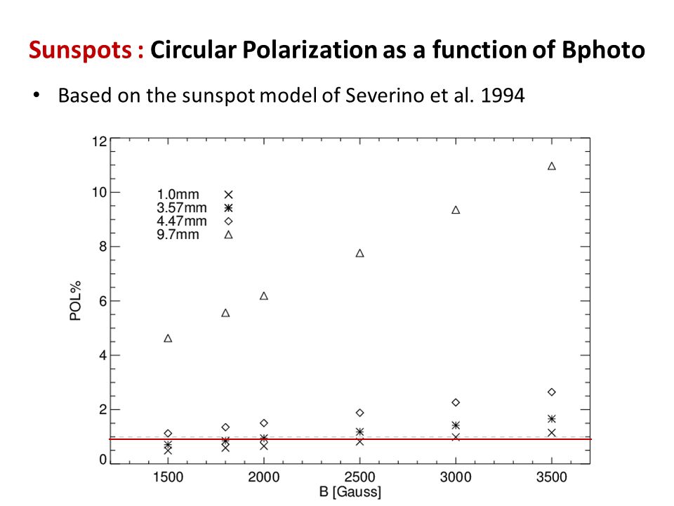
23. Sunspots : Circular Polarization as a function of Bphoto Based on the sunspot model of Severino et al. 1994