1. Data Description Chapter 3

2. The Focus of Chapter 3  Chapter 2 showed you how to organize and present data.  Chapter 3 will show you how to summarize data.  The primary method of doing this is to find the averages.  The word “average” is an ambiguous term.  In this chapter, “average” means measures of central tendency, specifically mean, median, mode and midrange.  Averages do not fully describe the data, we want to know how the data is dispersed. We will find measures such as range, variance and standard deviation.

3. Measures of Central Tendency 3 - 1

4. Parameters vs. Statistics  When the population is small it is not necessary to take a sample from the population in order gain information about the population. You can simply use data from all members of the population.  Parameters: Measures found by using all the data values in a population.  Statistics: Measures found by using data values from a sample of the population.

5. General Rounding Rule  In general, when calculating, rounding should NOT be done until the final answer is calculated.  Rounding in the middle of a calculation can tends to increase the difference between that answer and the exact one.  However, writing long decimals during computations may not be practical.  As such, you may round to three or four decimal places during calculations and still obtain the same answer that a calculator would give after rounding on the last step.

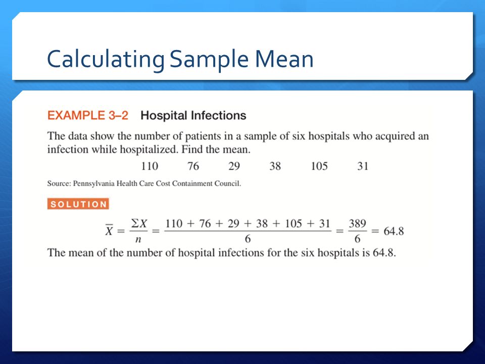
6. The Mean also called the arithmetic average. The Mean is found by adding the values of the data and dividing by the total number of values.

7. The Greek Symbol Sigma Σ  Σ means “sum”.  If we have data values {3, 2, 6, 5, 4} we can denote them in the following way.  ΣX means the sum of the X values.

8. Mean  Mean – The sum of the values divided by the total number of values.  Sample Mean – (denoted by, “X bar”) is calculated by using sample data. The sample mean is a statistic.  Population Mean – (denoted by μ, “mew”) is calculated by using all the values in the population. The population mean is a parameter. n = total number of values in the sample. N = total number of values in the population.

9. Rounding Rule for the Mean The mean should be rounded to one more decimal place than occurs in the raw data.

10. Calculating Sample Mean

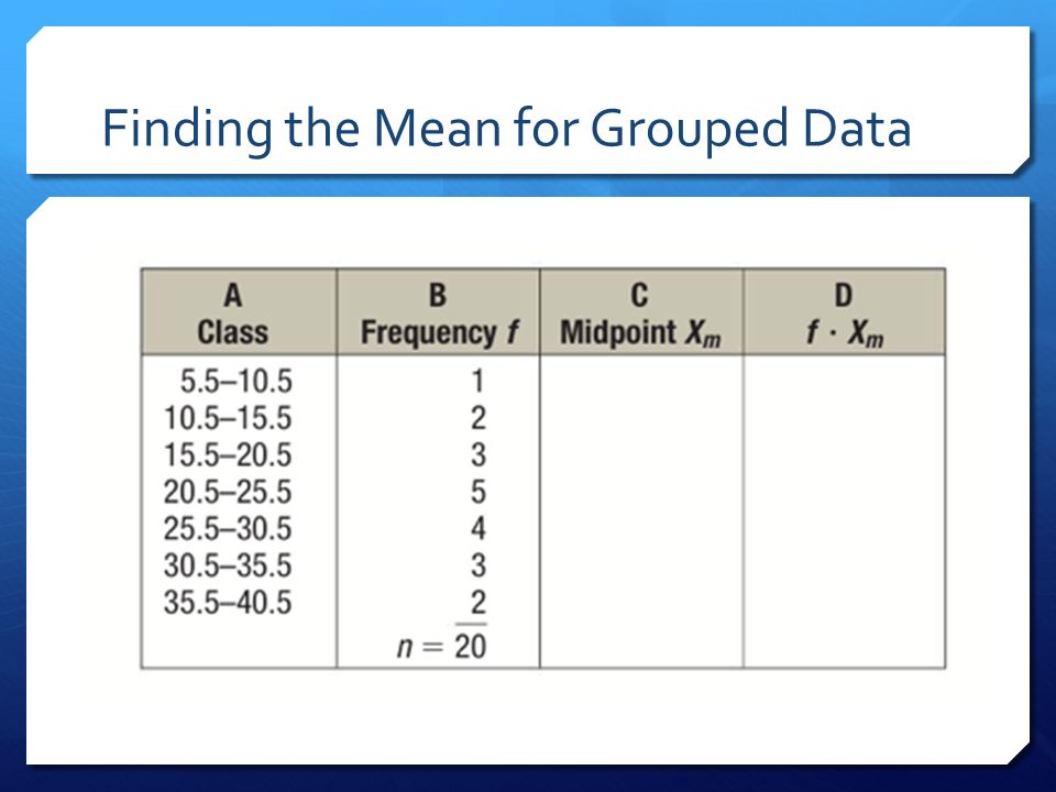
12. Finding the Mean for Grouped Data

14. The Median  The Median – is the midpoint of the data array. The symbol for median is MD.  Think of the median as the half way point of the data set.  A median of 86% on a test mean half the class did better than 86% and half the class did worse than 86%.

15. Calculating Median with an Odd Number of Data Values

16. Calculating Median with an Even Number of Data Values

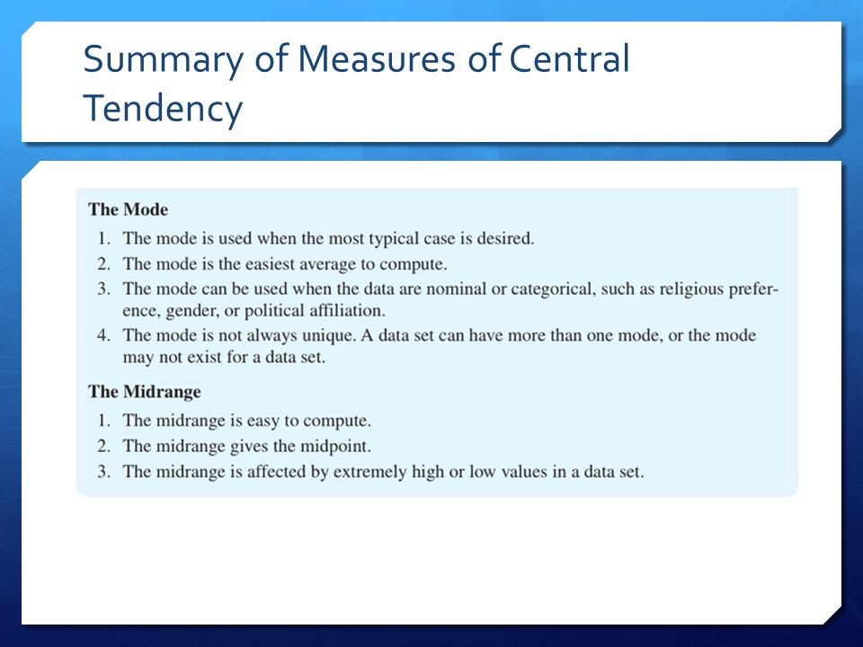
17. The Mode  Mode – the value that occurs most often in a data set.  Another word for mode is “the most typical case”  Unimodal – a data set with only one mode.  Bimodal – a data set with two modes.  This means two data values both occur with the same greatest frequency.  Multimodal – a data set with more than two modes.  This means each mode occurs with the same greatest frequency.  No Mode – When no data value occurs more than once.

18. Finding the Mode

19. A Bimodal Example

20. No Mode

21. Modal Class  The mode for grouped data is called the modal class.  The modal class is the class with the largest frequency.  Be aware that the mode or modal class is the only measure of central tendency that can be used in finding the most typical case when the data are nominal or categorical.

22. Modal Class of a Frequency Distribution

23. An Example of Finding Mode or Modal Class

24. The Effect of Outliers  Outliers – extremely high or extremely low data values in a data set.  Outliers can cause mean, median and mode for the same set of data values to be very different amounts.  An outlier can cause the mean to be much higher or much lower than the median or mode.  When outliers are present, the median may be a better measure of central tendency than the mean.

25. Example of the Effects of an Outlier

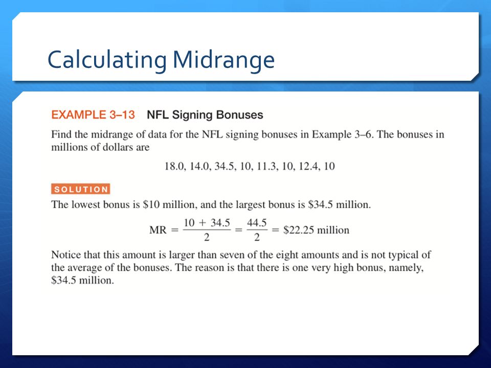
26. The Midrange  The midrange is a rough estimate of the middle.  The midrange is defined as the sum of the lowest and highest values in the data set, divided by 2.  The symbol for midrange is MR.

27. Calculating Midrange

29. Weighted Mean  A weighted mean is appropriate when the data values are not equally represented.  Consider three taxis that buy gas at three different gas stations at a cost of $3.22, $3.53 and $3.63 per gallon… The average of these three prices is…  However, the true average (mean) cost per gallon depends on how many gallons is purchased at each gas station.

30. Weighted Mean  A weighted mean is appropriate when the data values are not equally represented.  In the gas station example, the number of gallons purchased at each station is the “w” value.

31. Weighted Mean: Calculating GPA

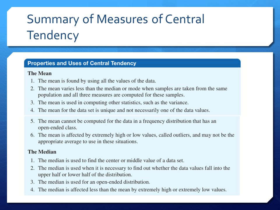
32. Summary of Measures of Central Tendency

35. Distribution Shapes  In a symmetric distribution, the data values are equally distributed on both sides of the mean.  When distribution is unimodal, the mean, median and mode are the same and are at the center of the distribution.  Examples are IQ scores or heights of adult males.

36. Distribution Shapes  In a positively skewed or right-skewed distribution the majority of data values fall to the left of the mean.  The “tail” is to the right.  The mode is to the left of the median.  The mean is to the right of the median.  An example is the incomes of the population of the U.S.

37. Distribution Shapes  A negatively skewed or left- skewed distribution occurs when the majority of the data values fall to the right of the mean.  The “tail” is to the left.  The mean is to the left of the median.  The mode is to the right of the median.  An example is test scores when most students have A’s and B’s but a couple students bomb the test.

38. An Example to Try…