1. Measurement of the CP Violation Parameter sin2  1 in B 0 d Meson Decays 6/15 Kentaro Negishi

2. Belle 実験 KEKB 加速器：電子 (e - )8.0GeV 、陽電子 (e + )3.5GeV 重心エネルギー 10.6GeV の非対称衝突型加速器 (10.6GeV = B 中間子一対がしきい値で生成 ) e - e + 衝突器として世界一のルミノシ ティ ピークルミノシティ :1.7×10 34 /cm 2 /s これまでに約 8 億個の B 中間子を生成 本論文でのデータは 10.5 fb -1 周長 3km ←  = 0.425

3. Belle 検出器はいくつかのサブ検出器からな る B 中間子の崩壊は Belle 検出器でとらえる

4. Spec of the Belle 3-layer SVD 50-layer CDC 1188 ACC 128 TOF 8736 CsI(Tl) crystals ECL 1.5 T 14-layer of 4.7-cm-thick iron KLM Resolution –Momentum for charged trk (  pt /p t ) 2 = (0.0019p t ) 2 + (0.0034) 2 p t [GeV] –Impact parameter  r  ~  z = 55  m –Specific ionization  dE/dx = 6.9 % (for minimum ionizing pions) –TOF flight-time  TOF = 95 ps –K ± identification efficiency ~ 85 %,  ± fake rate ~ 10 %, p < 3.5 GeV –Energy for  (  E /E) 2 = (0.013) 2 + (0.0007/E) 2 + (0.008/E 1/4 ) 2 E [GeV] E  > 20 MeV –e ± identification efficiency >90 %, hadron fake rate ~ 0.3 %, p > 1GeV –  ± identification efficiency >90 %, hadron fake rate 1GeV –K L angle 1.5° ~ 3°

5. Motivation The variable time-dependent asymmetry shows that the measurement of decays B 0 and B 0 to CP eigenstates is sensitive to  1.

6. Decay and subdecay mode  f = -1 –J/  (l + l - ) K S (  +  - ) –J/  (l + l - ) K S (  0  0 ) –  (2S)(l + l - ) K S (  +  - ) –  (2S)(J/   +  - ) K S (  +  - ) –  C1 (J/   ) K S (  +  - ) –  C (K + K -  0 ) K S (  +  - ) –  C (K S K -  + ) K S (  +  - )  f = +1 –J/  (l + l - )  0 –J/  (l + l - ) K L For the measurement of A(t), CP eigenstate mode is used.

7. Selection criteria J/ ,  (2S) →l + l - –opposite charged tracks are positively identified as lepton. –For J/  (l + l -  K S (  +  - ) mode, the requirement for one of the tracks is relax. – e + e - Including every g detected within 0.05 rad of e direction in invariant mass calculation. (radiative tail) Accept M J/ , M  (2S) [-12.5 , 3  ] (  ~ 12 MeV) –  +  - (radiative tail smaller than e + e - ) Accept M J/ , M  (2S) [-5 , 3  ] (  ~ 12 MeV)

8. K S →  +  - –The candidate is opposite charged track pairs that have an invariant mass within M KS [±4  ] (  ~ 4 MeV) K S →  0  0 –reconstructed from 4  within M KS [±3  ] (  ~ 9.3 MeV)  0 of the J/  0 mode –reconstructed from 2  lager than 100MeV within M  0 [±3  ] (  ~ 4.9 MeV)

9. Reconstruct of B (other than J/  K L ) M bc fit, after  E cut.  E selection depends on the each mode. (corresponding to ~ ±3  ) For M bc fit, the B signal region is defined as 5.270 < M bc < 5.290 GeV.

11. Reconstruction of J/  K L mode Requiring the observed K L direction to be within 45°from the direction expected for a two-body decay. Using likelihood fit for suppression of background. The likelihood depend on ↓ –J/  momentum at CM, –angle between K L and its nearest charged track, –multiplicity of the charged tracks, –The kinematics obtained by B + → J/  K* + hypothesis

12. Removing event that are reconstructed as –B 0 → J/  K S –B 0 → J/  K* 0 –B + → J/  K + –B + → J/  K* + In this mode, result is obtained as the p B cms distribution fit. p B cms calculated for B → J/  K L two-body decay hypothesis. The B signal region is defined as 0.2 ≦ p B cms ≦ 0.45 GeV

14. Identification of the B flavor Here, it is need to identify the B flavor. Tracks are selected in several categories that distinguish the b-flavor. l (p l high) from b → c l - l (p l low) from c → s l + K ± from b → c → s ; B0 → D ( ‘ ) → K ( ‘ )  (p  high) from B → D ( * )- (  +,  +, a 1 +, etc)  (p  low) from D* - → D 0  - Relative probability of b-flavor is determined by using MC, for each track in one of these categories. Combining the result ↑ to determine a b-flavor ‘q’. q = 1 : f tag is likely B 0 d q = -1 : f tag is likely B 0 d

15. Evaluating each event flavor-tagging dilution factor ‘r’ to correct for wrong-flavor assignment. The probabilities for an incorrect flavor assignment ‘w l ’ are measured by self-tagging mode reconstruction. w l are determined from the amplitudes of the time-dependent B 0 d -B 0 d mixing oscillations. r = 0 : no flavor discrimination r = 1 : perfect flavor assignment (N OF – N SF ) (N OF + N SF ) = (1 – 2w l )cos(  m d  t) N OF : number of opposite to tagged sample flavor events N SF : number of same flavor events

16. These tagging algorithm are verified to be a possible bias in the flavor tagging by measuring the effective tagging efficiency for B self-tagging samples, and different  t. Total effective tagging efficiency ⇔ good agreement with MC  l f l (1 – 2w l ) 2 = 0.2700.274 +0.021 -0.022

17. Determination of the  t The f CP vertex is determined by using lepton tracks (J/   (2S)) or prompt tracks (  C ). The f tag vertex is determined by tracks not assigned to f CP, and requirements (  r < 0.5 mm,  z < 1.8 mm,   z < 0.5 mm) –  r,  z are the distances of the closest approach to the f CP vertex in the r  plane, and z direction.   z is error of  z. The resolution function R(  t) is parameterized as a sum of two Gaussian. –SVD vertex resolution –charmed meson lifetimes –effect of B motion at CM –incompleteness of reconstructed tracks

18. The reliability of the  t determination and R(  t) parametrization is confirmed, and in good agreement with world average value. Algorithm OK

19. Determination of sin2  1 sin2  1 is obtained by an unbinned maximum- likelihood fitting to the observed  t distributions. Pdf for signal is –  B0d : B 0 d lifetime ~ (1.530 ± 0.009)10 -12 s –  m d : B 0 d mass difference ~ (0.507 ± 0.005)10 -12 ps -1

20. pdf for background is –f  : the fraction of the background –  bkg : effective lifetime –  (  t) : Dirac delta function –f CP modes, except J/  K L f  = 0.10  bkg = 1.75 ps –J/  K L mode J/  K*(K L  0 ) background pdf is fitted P sig with  f = -0.46 Non-CP background are fitted P bkg with f  = -1,  bkg =  B +0.11 -0.05 +1.15 -0.82

21. To obtain the likelihood value of each event as a function of sin2  1, the pdfs are convolved. f sig : probability that the event is signal

22. The most probable sin2  1 is defined as the value that maximizes the likelihood function L =  i L i.

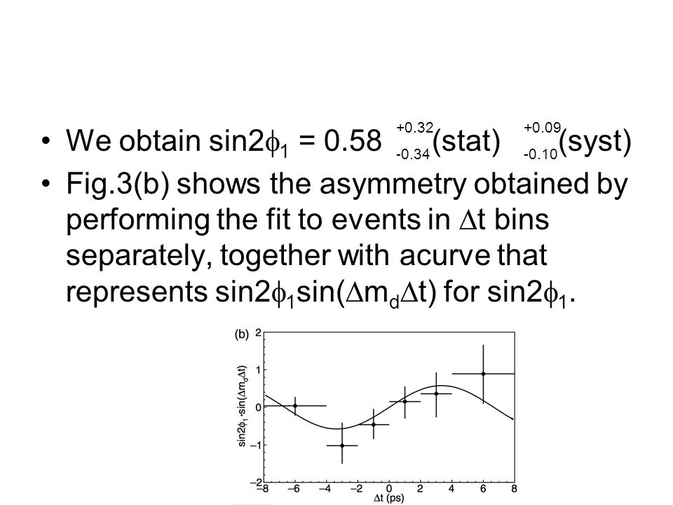
23. We obtain sin2  1 = 0.58 (stat) (syst) Fig.3(b) shows the asymmetry obtained by performing the fit to events in  t bins separately, together with acurve that represents sin2  1 sin(  m d  t) for sin2  1. +0.32 -0.34 +0.09 -0.10

24. Check for a possible fit bias by applying the same fit to non-CP eigenstates. –B 0 d → D ( * )-  + –B 0 d → D* -  + –B 0 d → J/  K* 0 (K +  - ) –B 0 d → D* - l + –B + → J/  K + It can not be possible to find asymmetry.

25. Summary Measurement of the standard model CP violation parameter sin2  1 based on 10.5 fb -1 data sample collected by Belle: sin2  1 = 0.58 (stat) (syst) +0.32 -0.34 +0.09 -0.10